


Deriving some numerical integration formulas
Party like it's 1814

I’ll assume that you know that the definite integral of a function from a to b gives the area under the function’s curve between x = a and x = b, and that you can integrate polynomials.1 Sometimes you need to integrate a function over an interval and you don’t know the anti-derivative, and at these times you make the computer calculate a number for you. This post derives increasingly sophisticated ways that you might program a computer to do the calculation, without assuming knowledge of sophisticated underlying mathematics.
All of the methods will involve dividing the interval into pieces, approximating the area for each piece, and adding up the areas. The first section covers simple methods in which the function is evaluated at regular intervals; these were part of my year 12 curriculum. The second section, which is the real purpose of this post, derives some integration schemes (Gauss and Gauss-Kronrod) in which the function is evaluated at specially chosen, unevenly spaced points, the results carefully weighted to give the final approximate area.
Even these latter intimidating methods turn out to be explicable from elementary principles, accessible in some sense to an advanced high school student, albeit involving an enormous quantity of algebra more suited to a third- or fourth-year uni course. My naive (and perhaps bumbling) approach is absolutely not how the relevant parameters are computed for serious integration libraries such as QUADPACK. But I calculate the necessary parameters to nine or ten correct digits, indicating that my basic ideas are sound, even if the implementation is not appropriate for high-precision computing.
I’ll only consider well-behaved functions f over a finite interval [a, b], and I won’t derive any theoretical error bounds, which is a boring topic. If you want an approximate error, just halve the size of your pieces and see how the computed integral changes when you do the calculation again.
1. Simple methods
1.1 Rectangular
Don’t overthink it: approximate the area under the curve by a bunch of rectangles.
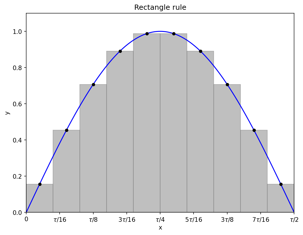
If we have N rectangles each of width Δx, then Δx = (b − a)/N, and we need to evaluate the function at points
from n = 1 to n = N, the subtraction of one half being required to get the point in the middle of each rectangle.
The area of rectangle n is the width Δx times the height f(x_n), so the approximate integral is
The ten rectangles in the diagram above represent an approximation to the integral
and their combined area is about 2.008, pretty close to the exact integral, which is 2.
1.2 Trapezoidal
Curves are, in general, not horizontal, so perhaps we can do better by approximating the curve by trapeziums (it doesn’t actually help much, if any):
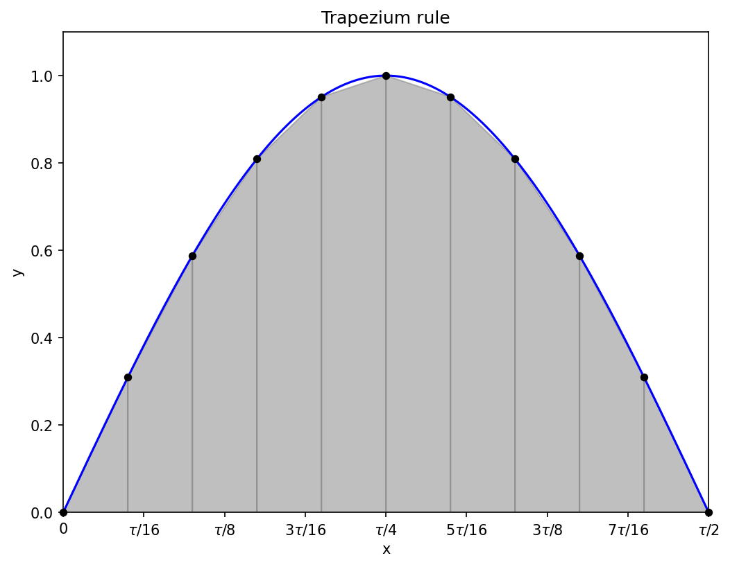
Now we need to evaluate the function at the end-points of each sub-interval (rather than the mid-points needed for the rectangles), so for N trapeziums there will be N + 1 function evaluations, at2
The area of trapezium n is
and each f(x_n), except the first and the last, contributes to two trapezium areas. The final rule is therefore
The bulk of the calculation is equally-weighted function evaluations every Δx, very similar to the rectangle rule, just with the points offset by half the interval widths, and some corrections at the end-points. The much-improved visuals do not actually lead to a major change in the accuracy of the integral.
Note that errors will all accumulate on one side if the curve is consistently concave up or concave down, as can be seen near the peak of the sine wave above: all the trapezium approximations under-estimate the function. The estimated integral from the 11 function evaluations in the diagram is about 1.984, noticeably less accurate than the rectangles.
1.3 Simpson’s rule
Curves are, in general, not piecewise-linear, so perhaps we can do better by approximating the curve by quadratics (this usually helps a lot with smooth functions):
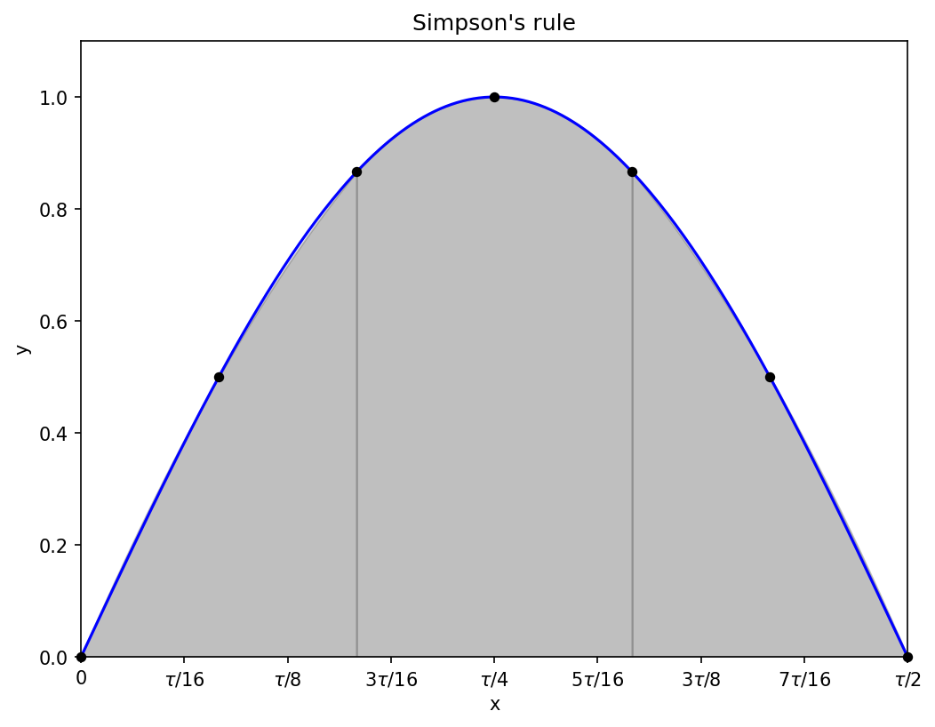
Even with a reduced number of points compared to the earlier rules, the parabolic approximations to the sine wave are excellent, and you can barely see the difference between the shaded region and the blue curve.
We can use the same definitions of x_n and N as for the trapezium rule, but now we require that N is even: where there were previously two trapeziums, there is now one quadratic covering a sub-interval of width 2Δx; the three points are sufficient to uniquely define the parabola.
What is the area under one of these quadratics? First, let’s shift the sub-interval so that it goes from x = −Δx to x = +Δx; the area won’t change if we move it left or right, and having the sub-interval be symmetric around x = 0 simplifies the maths.
Write the quadratic approximation p(x) as
we will need to find the coefficients in terms of f(−Δx), f(0), and f(Δx). In fact we will only need two of the coefficients, because the linear term, being odd, does not contribute to the integral (a first useful consequence of centering the sub-interval around x = 0):
The three points give the equations
The middle equation immediately gives the constant term (a second useful consequence of centering the sub-interval around x = 0). Adding the first and third equations eliminates a_1, so that
or
Substituting into (2) gives the integral of p(x) in terms of the function values,
This is now in a form ready for use in deriving the integration formula, known as Simpson’s rule. Remember from (1) that I’m using 1-based indexing for my points, so that x_1 is at the lower bound of the interval to be integrated. The even-indexed points will all be in the middle of a sub-interval approximated by one quadratic, so they will all have their function evaluations multiplied by 4/3. The odd-indexed points, except the first and the last, will each be an end-point of two sub-intervals, and will therefore have their function evaluations multiplied by 2/3.
The multipliers for the function evaluations therefore go 1/3, 4/3, 2/3, 4/3, 2/3, 4/3, …, 2/3, 4/3, 1/3, alternating between 2/3 and 4/3 except at the end-points. Even though I have already explained why, I find it somewhat surprising that such alternation either side of 1 often leads to more accurate numerical integrals than consistently using 1 as in the trapezium rule.
Written as a single formula, Simpson’s rule is
With nine function evaluations (four sub-intervals approximated by a quadratic), the estimated integral of the half-period sine wave is about 2.0003, an extra correct digit or two compared to the rectangles and trapeziums.
Adaptive sub-interval widths
So far I’ve assumed that the widths of all the sub-intervals are a constant Δx. It’s possible instead to have varying widths, going to narrower sub-intervals in places where the approximation error is estimated to be high. I’ll bypass adaptive algorithms for now, leaving it for a method below (Gauss-Kronrod) which is explicitly designed for this framework.
2. Fancy methods
In a fancy numerical integration method, we take evaluate the function at specific points within the interval to be integrated, multiply each value by a specific weight, and add up the results. In this section, I will always use the interval [−1, 1] when doing the algebra; intervals of other lengths just need a scaling factor.
In applications, we will often, as previously, need to split the whole interval into many sub-intervals to get a good approximation, repeating the calculation on each sub-interval. But hopefully the total number of function evaluations needed for a given approximation error is less than when using one of the simple methods.
In terms of symbols, we want to choose N points x_n with weights w_n such that
is a good approximation.
If you’re anything like me, then you’ve been mildly interested in how this works for a long time, but you’ve never sat down and learned it. There are two likely causes of this inaction:
All of the relevant Wikipedia articles have titles that end with ‘quadrature’, which is a big and scary word. While you wouldn’t admit this in public, you aren’t really sure what it means.
If you nevertheless click on one of those articles, you get half-way through the introduction before tapping out at “roots of the nth Legendre polynomial”.
It turns out that quadrature is just numerical integration, and you can get a long way without needing to learn what a Legendre polynomial is.
2.1 Gauss
Let’s say we would like to define an N-point integration rule: we get to choose N values of x_n and N weights w_n. The goal of the Gauss-based integration rules is to make these choices so that all polynomials of degree M passing through the selected points will have their integrals computed exactly, for the maximal possible choice of M.
It is very plausible that this will lead to accurate approximations of integrals, because a high-degree polynomial can give a close approximation to quite nonlinear functions. In the following example, four full periods of a sine-wave over [−1, 1] are approximated pixel-perfectly by a polynomial of degree 19.
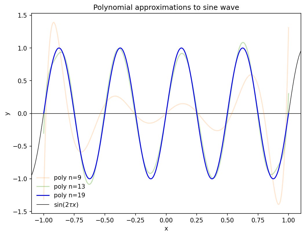
How to find such a polynomial approximation is beyond the scope of this post.3
Working with high-degree polynomials is sometimes dangerous, and showing why Gaussian quadrature avoids such danger is also beyond the scope of this post.4 The motivation for the derivations that follow remains the plausible assumption that the approximations should be good.
At first glance we might think – I certainly thought – that the maximal degree M must necessarily be one less than the number of points, i.e. M = N − 1. A polynomial of degree N − 1 has N coefficients (including the constant term), and all N points would be necessary to generate enough equations to solve for them.
But odd powers of x are anti-symmetric around x = 0, so their integrals over [−1, 1] are all zero. This means that we don’t need to solve for the coefficients of odd-power terms, opening up the possibility of getting the polynomial integrals correct up to degree M = 2N − 1.
Gauss computed the positions and weights for up to N = 7 (section 22 here has the summary tables5); let us, if not precisely follow in his footsteps, then at least walk to the same destination. The algebra builds in complexity as the number of points increases. I will studiously ignore the work of Jacobi, which I gather from Wikipedia is the foundation of modern treatments of this subject.
N = 1
We won’t get very far with one point: M = 2 × 1 − 1 = 1. It is not surprising that we need to put the point at the centre of the interval at x = 0, but let’s see how to derive it formally; similar ideas will be used as we increase the number of points.
We want to exactly integrate all linear functions with our one point, so define
The desired integral is
and we would therefore like to choose a point x_1 and a weight w_1 such that
We substitute in our linear function on the left-hand side to get
We require this equation to hold for all possible choices of a_0 and a_1, so we equate like terms (i.e., the coefficients in equation (4) of the coefficients a_0 and a_1 of the linear polynomial defined in (3)):
The 1-point Gauss rule indeed says to evaluate the function at the mid-point of the interval, giving it a weight of 2, the width of the interval. This is just the rectangular rule.
N = 2
With two points, we can integrate all polynomials up to degree 3. Write
and note that the desired integral is
We want to choose x_1, x_2, w_1, and w_2 such that
We equate the coefficients of the a_i. The odd-indexed coefficients must be zero, which enforces the expected symmetries of x_1 = −x_2 and w_1 = w_2. That leaves the equations coming from the even-indexed coefficients,
so that each of the two weights is 1, and the x-values are ±1/√(3) ≈ ±0.577.
If you divide an interval into many regular sub-intervals and apply the two-point Gauss rule on each, then the calculation looks similar to the rectangular rule in that each point is given the same weight, but the Gauss points are slightly closer together or further apart:
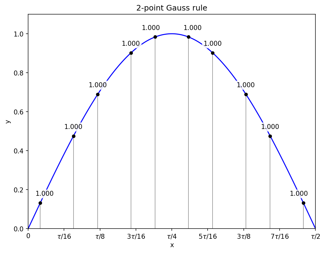
The above diagram contains five sub-intervals, for ten function evaluations, and these lead to an estimated integral of about 1.99993, closer to the exact value than Simpson’s rule with 11 function evaluations (2.0001), and much closer than the rectangular rule (2.008).
I find it deeply surprising that an equal-weighted sum of function evaluations is substantially improved by breaking the symmetry of a regular discretisation. I do not have an intuition for it, only the mechanical explanation provided by the algebra.
N = 3
From here on I’ll ignore the odd terms and just automatically enforce symmetry conditions. With three points, we can label x_2 = 0 and x_1 = −x_3, with w_1 = w_3. The fourth-degree polynomial is
which has the integral
Equating like terms in the expansion of
leads to the equations
Substituting the second equation into the third gives
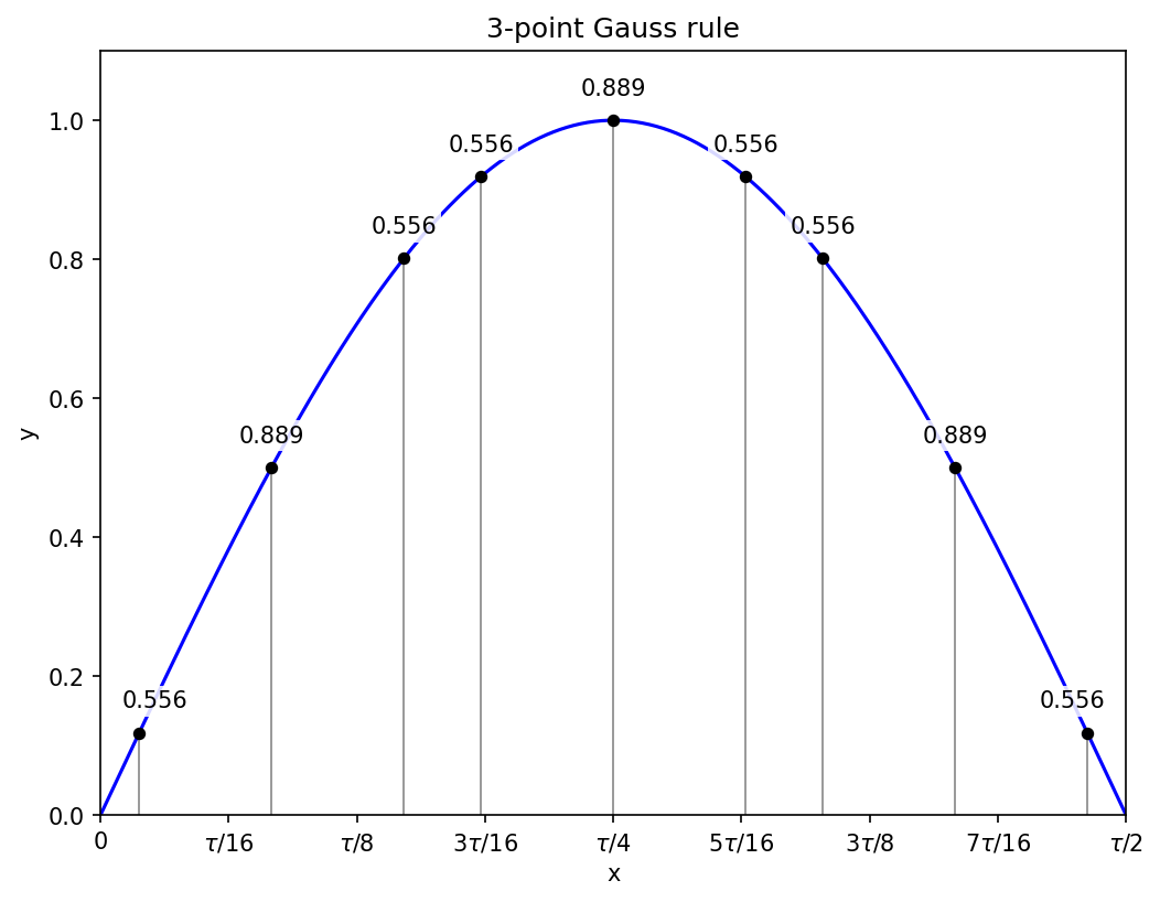
and then w_1 = 5/9 and w_2 = 8/9.
Three sub-intervals and hence nine function evaluations get the sine integral correct to within 1.4e-6.
N = 4
With four points we need to solve for two positions and two weights, the others following from symmetry. Similar reasoning to the above cases leads to the system of equations
I’ll change notation to
for tidiness. The system of equations in terms of these new variables is
My imagined reader who is an advanced high school student will probably struggle to solve this system unaided. That is what I tell myself anyway; I scratched away at it for a while before giving up and asking o3-mini-high, whose solution I will now adapt.
The key idea, which I will use in some form for every derivation in the rest of this post, is to get a recurrence relation involving ax^n + by^n expressions for different values of n. Multiplying such an expression by x + y gives
which rearranges to
Since we have the values of ax^n + by^n for n = 0 to 3 from equations (5) to (8), we can use the recurrence relation to convert the starting system of equations into a pair of equations for new variables (x + y) and xy. Equation (7) gives (using (6) and (5))
Similarly, equation (8) now becomes (using (7) and (6))
Solving the simultaneous equations (9) and (10) for the sum and product variables is straightforward, the solutions being
Using y = 3/(35x) from the first equation and substituting into the second gives a quadratic in x,
which has the solutions
Recalling that x is the square of the position, the final locations of the Gauss points are
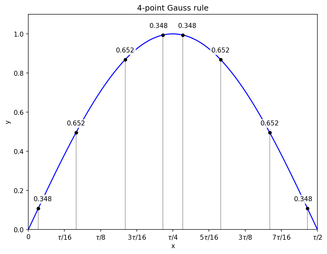
and their symmetric negative counterparts. Equations (5) and (6) are now a linear system in the weights, with the solution
Two sub-intervals and hence eight function evaluations get the sine integral correct to within 4.6e-8.
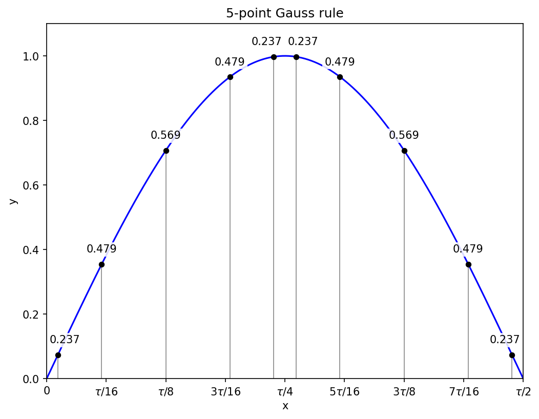
N = 5
With five points, symmetry requires that one is at x = 0, and the others come in plus-or-minus pairs. The equations for the positions are therefore structurally identical to those in the N = 4 case, though the numbers change because we now apply the recurrence relation one degree higher. Using a similar notation, with c denoting the weight of the x = 0 point, the equations to solve are
Applying the recurrence relation to the last two of those equations gives two equations in (x + y) and xy:
These have the solution x + y = 10/9 and xy = 5/21, leading to a quadratic equation for x of
and after taking the square root of the solutions, we have the non-zero Gauss point positions as
Given the positions, the weights are the solution to a system of two linear equations, straightforward albeit a little tedious to do by hand.
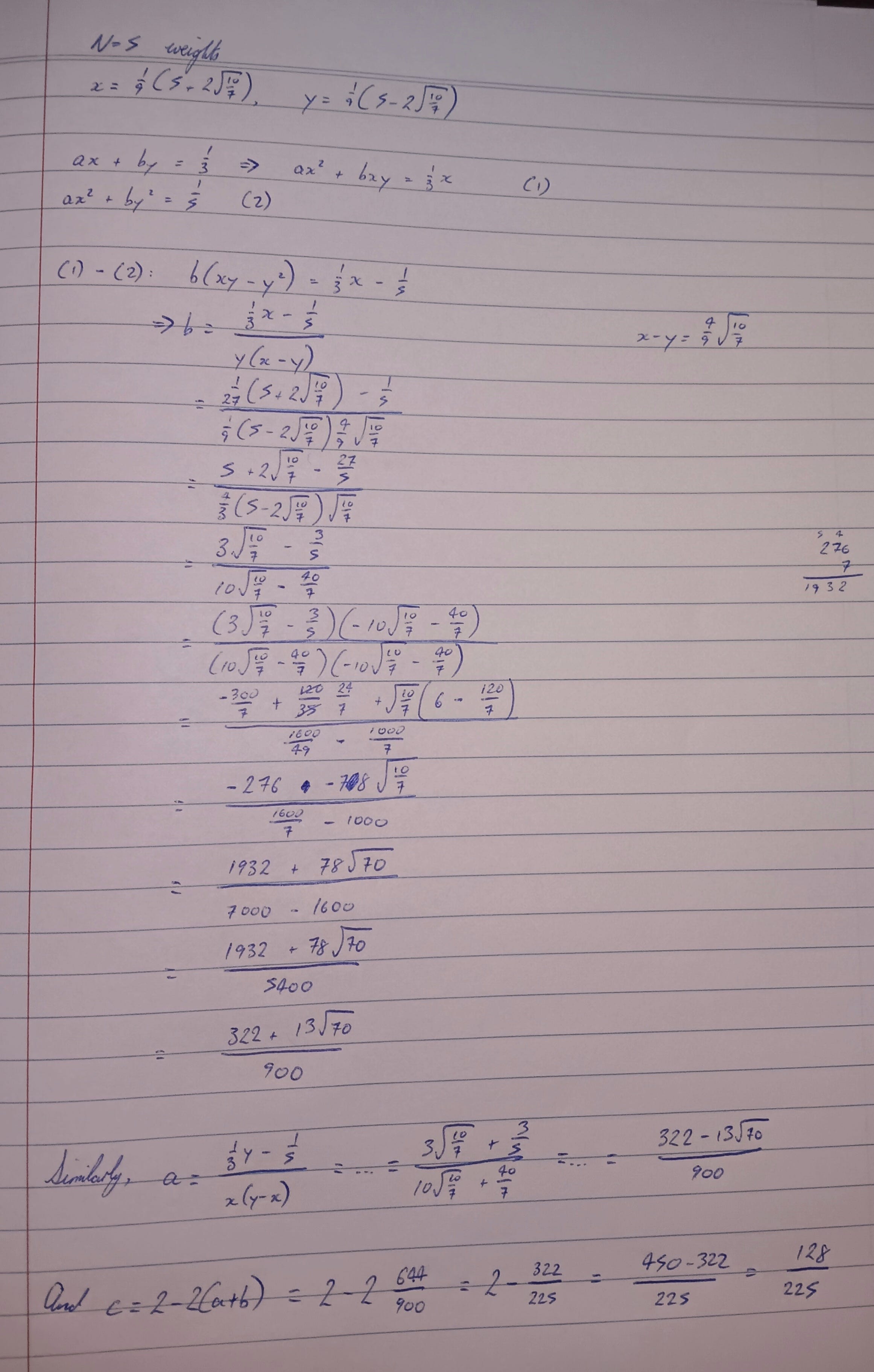
Two sub-intervals and hence ten function evaluations get the sine integral correct to within 8e-11.
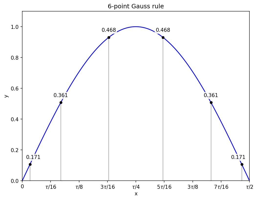
N = 6
Now there are three positions to solve for, and I’m pleased to report that I didn’t need AI assistance to generalise the recurrence relation to the three-variable case, and eventually work my way to a cubic equation in p = xy (the product of the squares of two of the positions). This may not be the most direct approach, but it was the one I found, and it works.
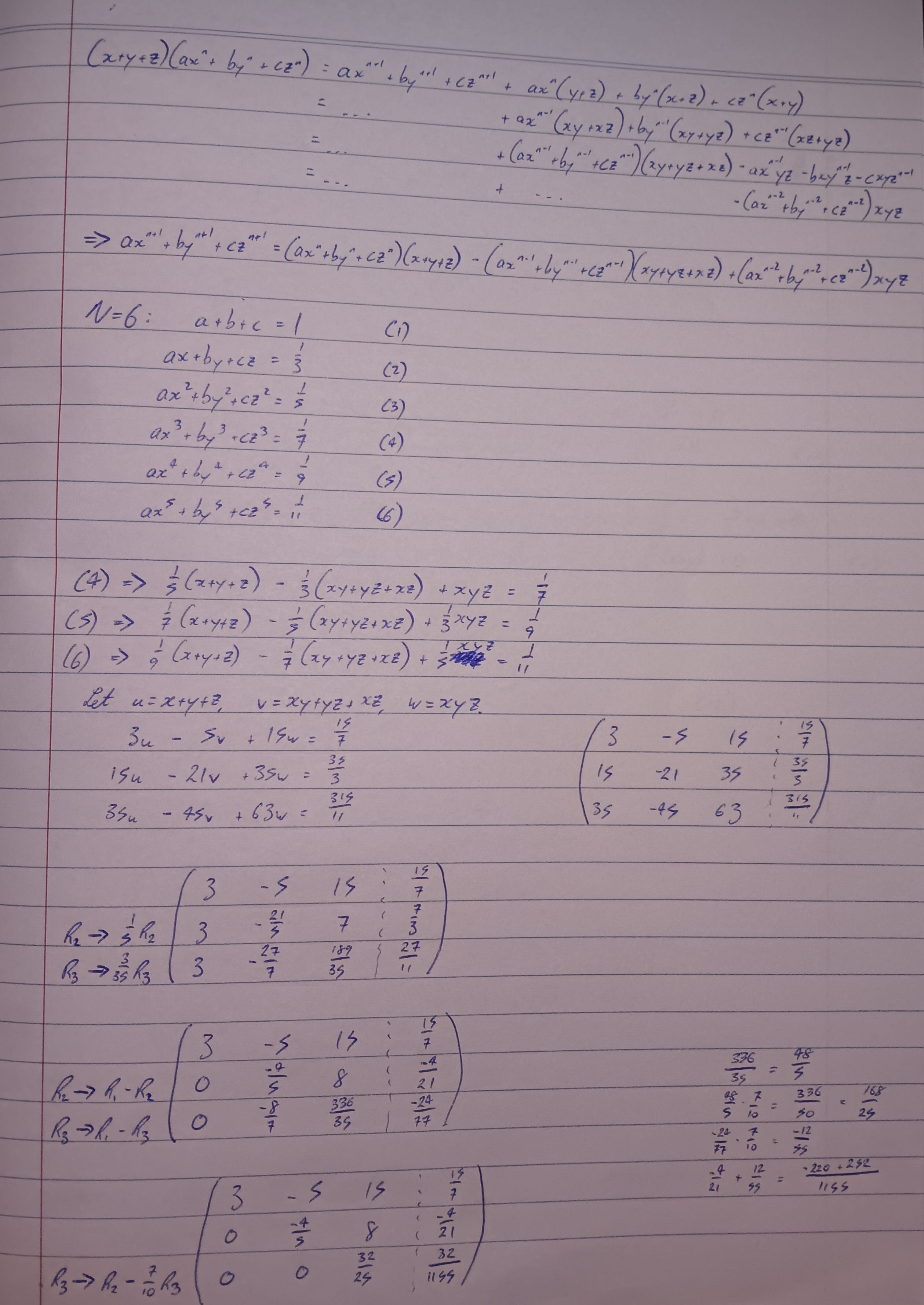
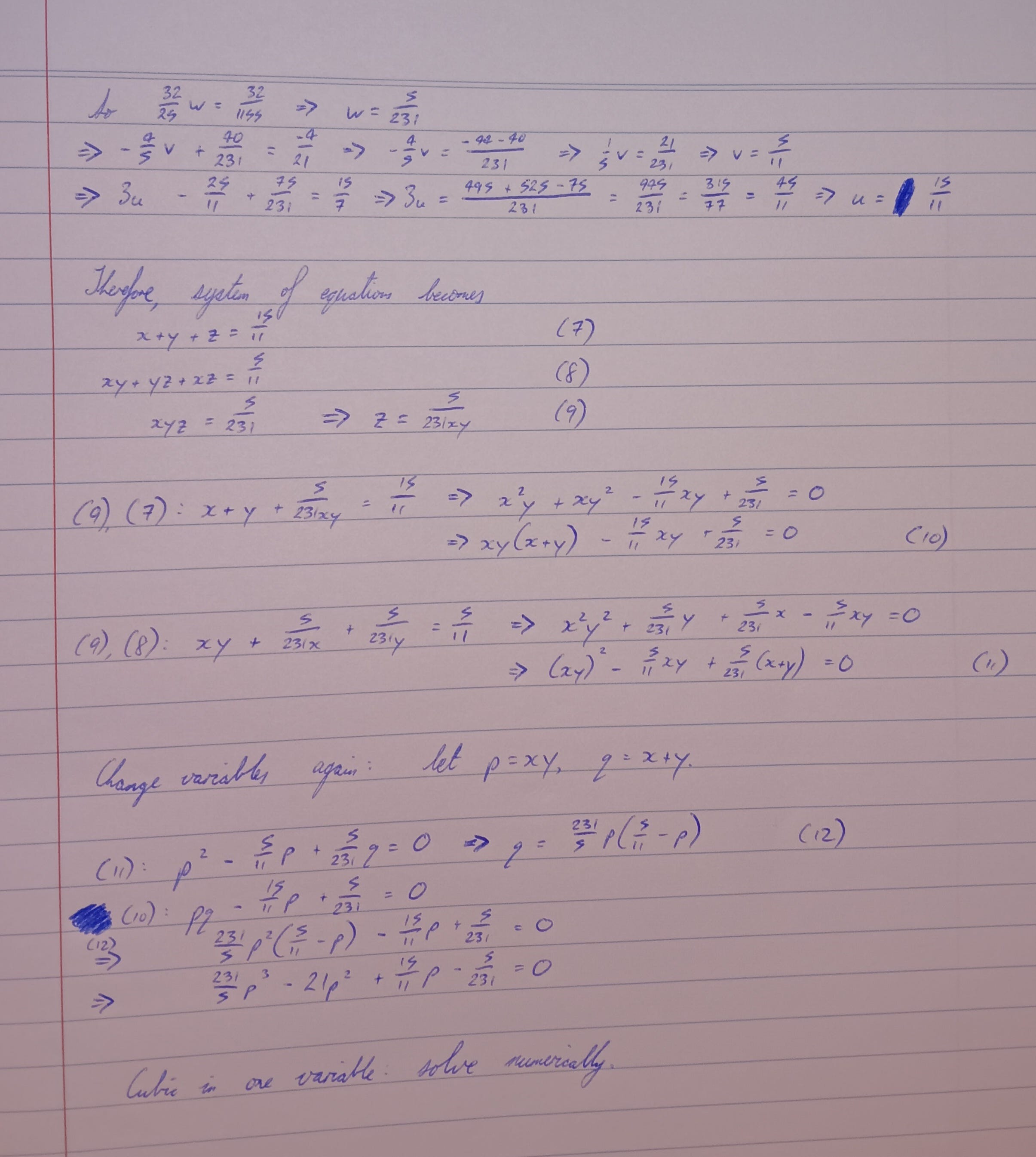
At this point I think it is reasonable to switch to silicon. Gauss could have painstakingly approximated the roots of the cubic by hand, and given enough hours I could do likewise. I am just using the computer to speed things up.6
The equation is
and the solutions are
The corresponding sums q = x + y can then be computed from my handwritten equation (12),
namely
The sum and product define a quadratic for x with solutions
the “plus or minus” giving two out of the three squared positions. Taking the square roots to get back to the original scale defines the Gauss points as
and their symmetric negative counterparts.
Any three of the initial set of equations can then be used to define a linear system for the weights, which are
Applying the six-point rule on the full interval [0, tau/2] gets the sine integral correct to within 5.6e-11.
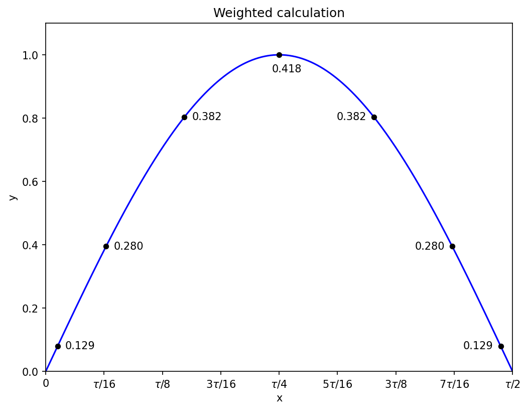
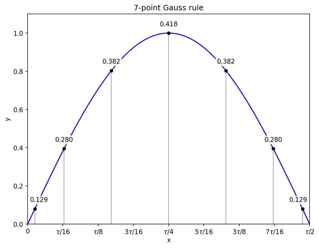
N = 7
Just as the calculation for N = 5 is similar to N = 4, the calculation for N = 7 is similar to N = 6: one of the points will be at x = 0, and the other six will come in symmetric pairs, so there are three unknowns for the positions, and the equations will lead to a cubic.
Having satisfied myself during N = 6 that I can do the relevant algebra, I got the computer to solve things for me in the way that I would have worked by hand, since all that changes from N = 6 is the arithmetic. The starting equations are
Applying the recurrence relation leads to a new system of equations that resolves to
These in turn lead to a numerically-solved cubic equation in the product p = xy,
and we get the sum x + y from
The sum and product define a quadratic equation for the squares of the positions, and working through the cases and taking square roots gives the positions of the non-zero Gauss points as
along with their symmetric negative counterparts. The corresponding weights are
with the point at x = 0 getting the largest weight, approximately 0.417959183673.
Applying the seven-point rule on the full interval [0, tau/2] gets the sine integral correct to within 1.8e-12.
Mini-conclusion
I have found this a satisfying exercise. Gauss had more mathematical insight than I have, but he wasn’t doing magic. He had a key idea about how you could integrate numerically and he doggedly pursued it to its conclusion. I feel now the way I felt after writing my post on the Fast Fourier Transform: slightly less awed by Gauss.

I only have another hundred or two major breakthroughs by Gauss left to understand.
2.2 Adaptive sub-intervals and Gauss-Kronrod
A function may vary rapidly in some places, requiring quite fine discretisations to integrate accurately, and be more gentle in others, where coarser sub-intervals can be used with little error.
Suppose that we have a function called INTEGRATE which takes the interval to integrate as an argument, and returns the estimated integral and error; this error is always given as an absolute value, never negative. Then we can use the following sketched algorithm to adapt the sub-intervals as needed to get the estimated error for the whole interval below some tolerance.
Call
INTEGRATEover the full interval, setting variablesintegralanderrorto the results.If the error is less than the tolerance, then return
integral.If we reach this step, then the error was not below the tolerance, and we do the adaptive algorithm. Initialise a list that will contain the sub-intervals and their corresponding integrals and errors. The first element will be the full interval with the integral and error just computed.
Loop:
Find the list index i which contains the maximum error.
Define two new sub-intervals by splitting sub-interval
iinto two.Call
INTEGRATEon the two new sub-intervals, and append the results to the end of the list.Update
integralanderrorby subtracting the results of the old sub-intervaliand adding the results from the new sub-intervals.Remove the old sub-interval from the list.
If
erroris less than the tolerance, then returnintegral.
In reality you would probably terminate the loop after some specified maximum number of iterations, just in case something bad is happening in the error is not falling below the tolerance.
The challenge is that the Gaussian quadrature formulas just give us the approximate integral, not an estimated error. A naive way to estimate the error would be to re-do the Gaussian quadrature using sub-intervals of either twice or half the size (depending on your perspective), and then compare the results. Since we would return the result from the finer discretisation, the calculation of the error by this method involves doing an extra 50% function evaluations compared to the calculation of the integral alone.
Function evaluations are often the slowest part of the calculation: multiplying two numbers (weight and function value) is fast, but the function may have trig functions or exponentials or divisions etc., which take longer to compute.
Kronrod’s idea was to allow the error estimate, similar in spirit to redoing the calculation at half/double resolution, to be incorporated into the same set of function evaluations:
Evaluate the function at the N Gauss points and compute the integral by the N-point Gauss rule.
Insert N + 1 Kronrod points in between the Gauss nodes, and compute the integral using the (2N + 1)-point Kronrod rule.
The Kronrod part of the calculation involves a new set of weights that applies to both the Gauss points and the new Kronrod points. The Kronrod points are located, and the weights chosen, so that all polynomials up to a maximal degree passing through the points are integrated exactly.
Since the Gauss points are optimised for an N-point calculation rather than a (2N + 1)-point calculation, we will not be able to reach degree 4N + 1. We have N + 1 free points to work with and 2N + 1 weights, so we can reach degree 3N + 1.
The 7-point Gauss rule becomes associated with a 15-point Kronrod rule, and Wikipedia gives the points and weights for this G7, K15 case. It is surprisingly difficult to find references for other choices. (This is in contrast to Gaussian quadrature without Kronrod, for which there is a wonderful webpage covering up to N = 64.)
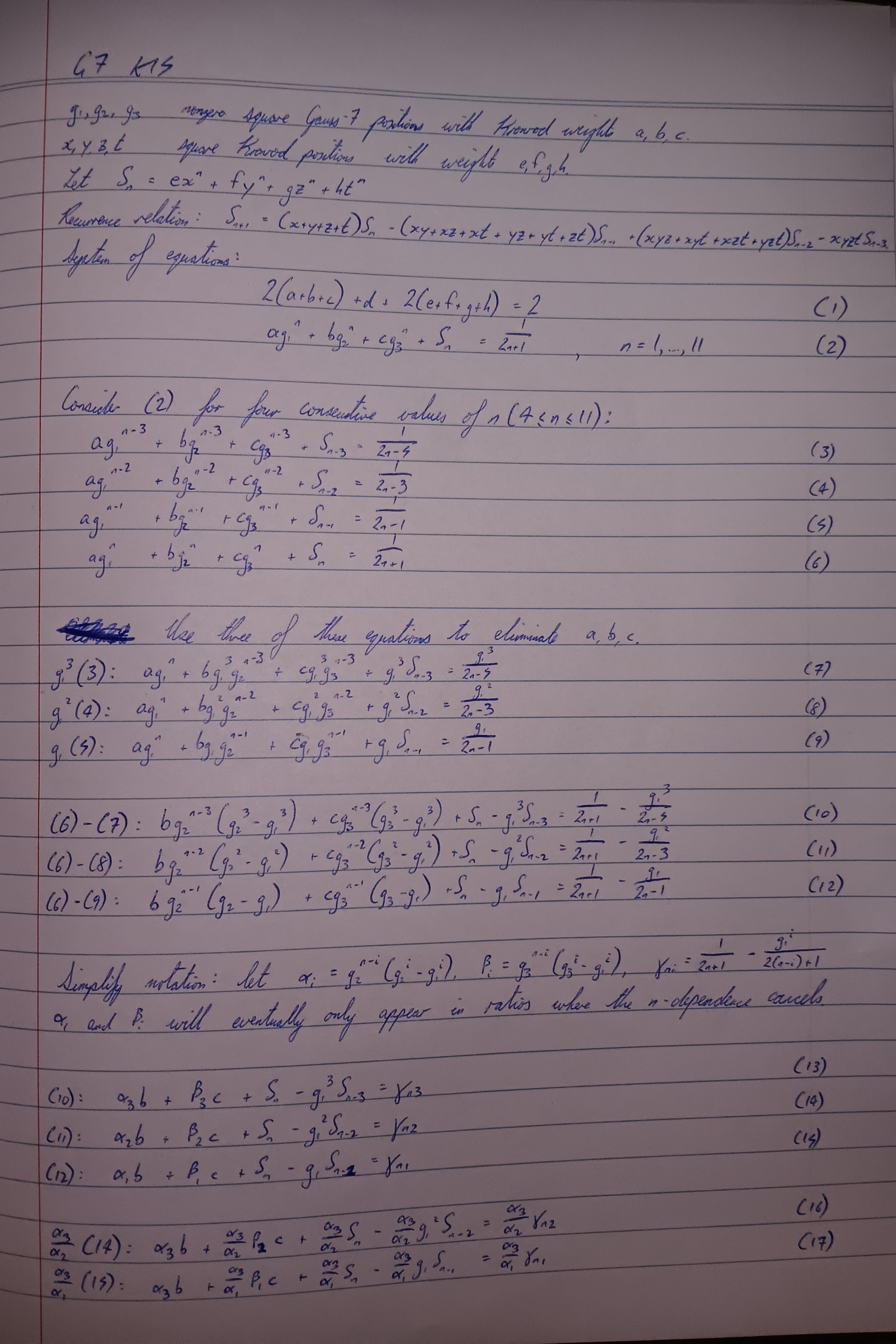
I will not laboriously derive (G2, K5), (G3, K7), etc. – this post is long enough as is. I will instead jump straight to (G7, K15); earlier cases are simpler versions.
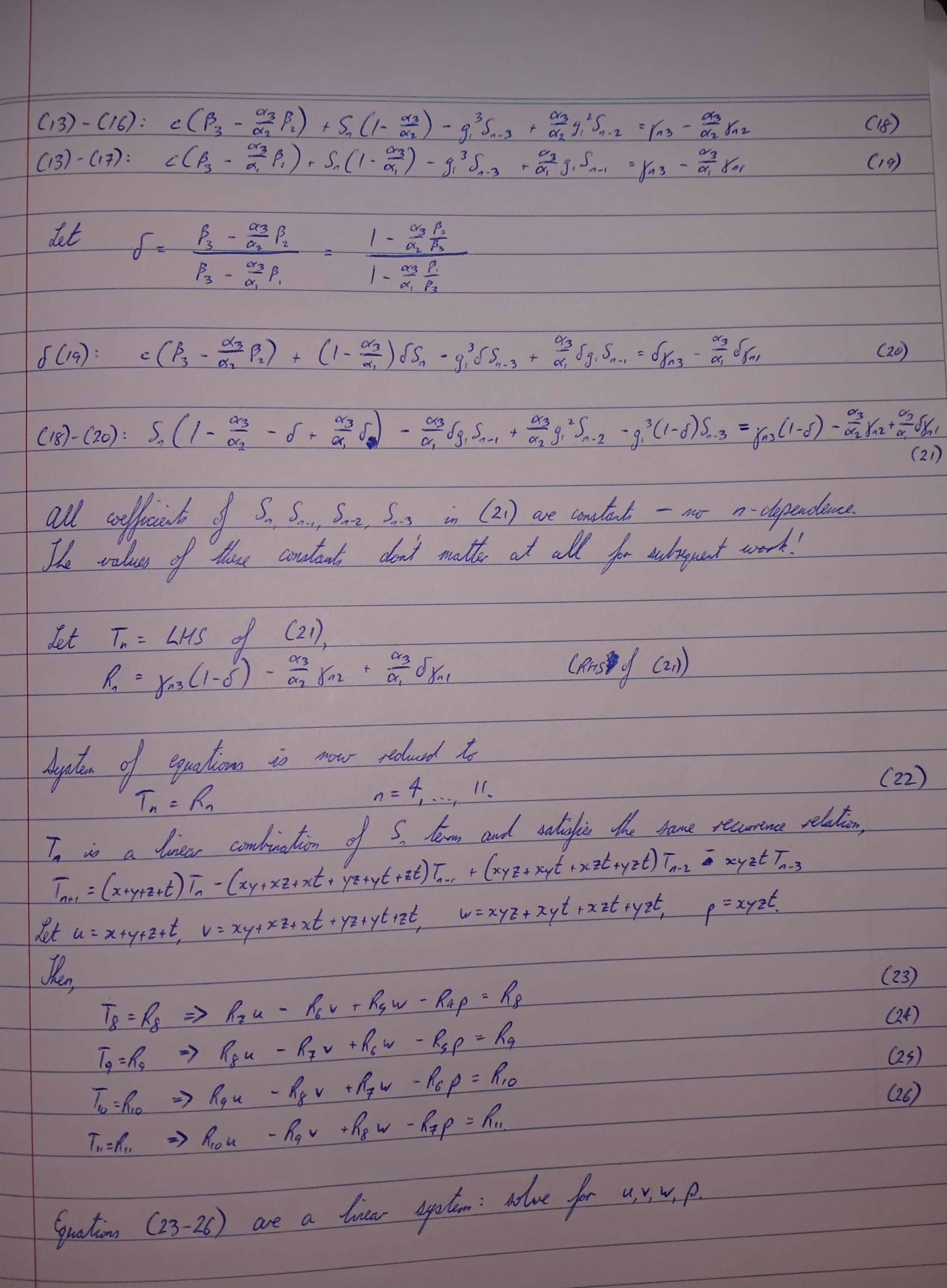
Let g_1, g_2, and g_3 be the squares of the nonzero Gauss-7 points, with Kronrod weights (to solve for) of a, b, and c; let d be the weight of the Gauss point at zero. Let x, y, z, and t be the squares of the Kronrod points, with weights e, f, g, h. After enforcing symmetries, we are left with a system of 12 equations:
Kronrod was working in the 1960’s, which is in the computer era. So I decided not to work through pages of algebra again, instead just giving the equations and some rough initial guesses to scipy.optimize.fsolve, which quickly converges to The iteration is not making good progress, as measured by the improvement from the last ten iterations.

Pen and paper it is.
Once again there is some theory that I am going to obstinately not learn. “These extra points are the zeros of Stieltjes polynomials”? A statement dreamed up by the utterly Deranged.
I have one tool at my disposal – the moment recurrence relations – and I am going to plough straight ahead with it.7
The first equation (sum of weights) will be left to the end, only used to find the weight of the Gauss point at x = 0. That leaves 11 equations to work with.
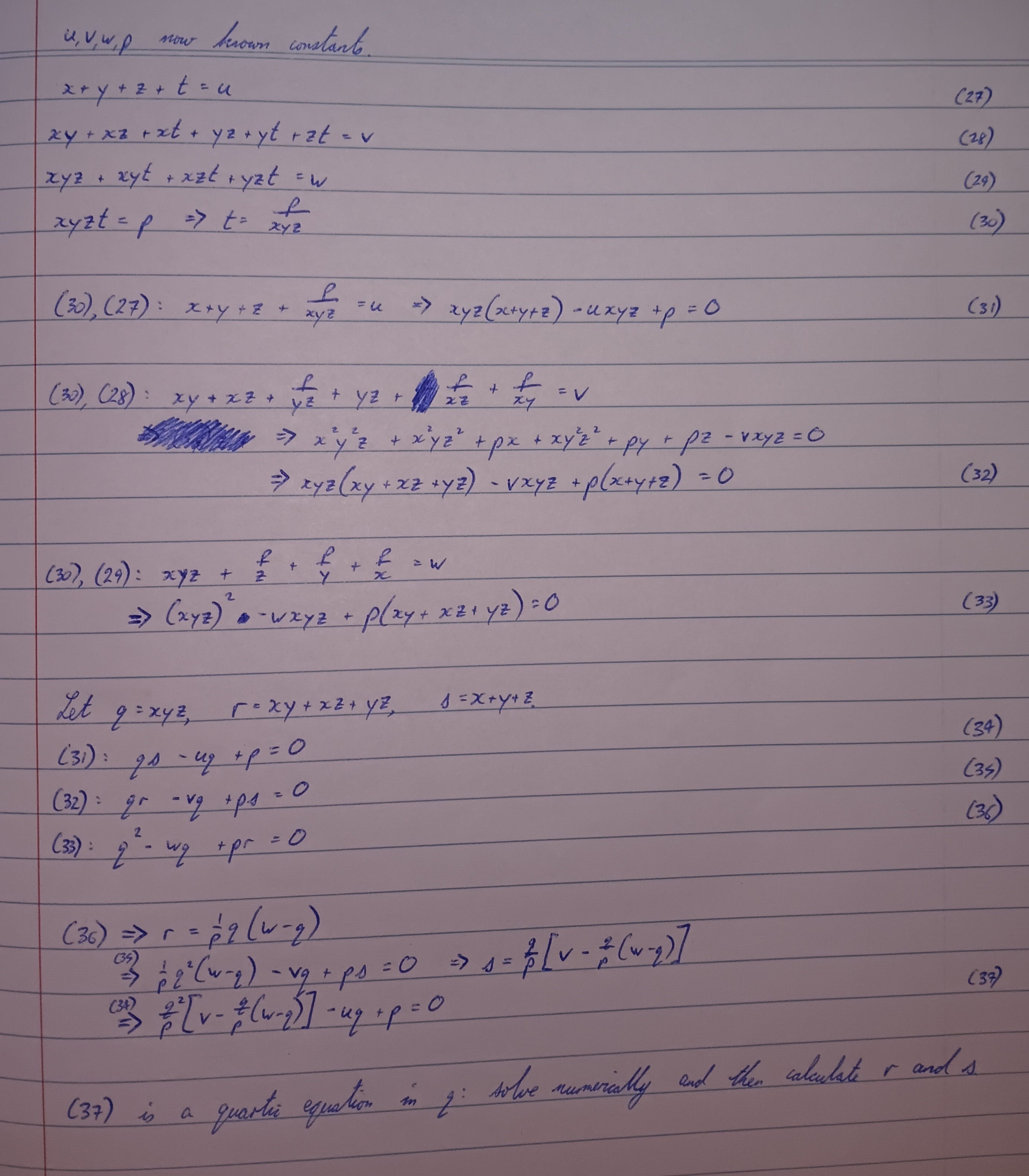
The strategy is to first eliminate the Gauss-point weights a, b, and c, reducing the 11 equations down to 8. Applying the four-point recurrence relation then leads to a linear system of four equations in four variables (sums and products of x, y, z, t), whose solution reduces to a quartic in xyz.
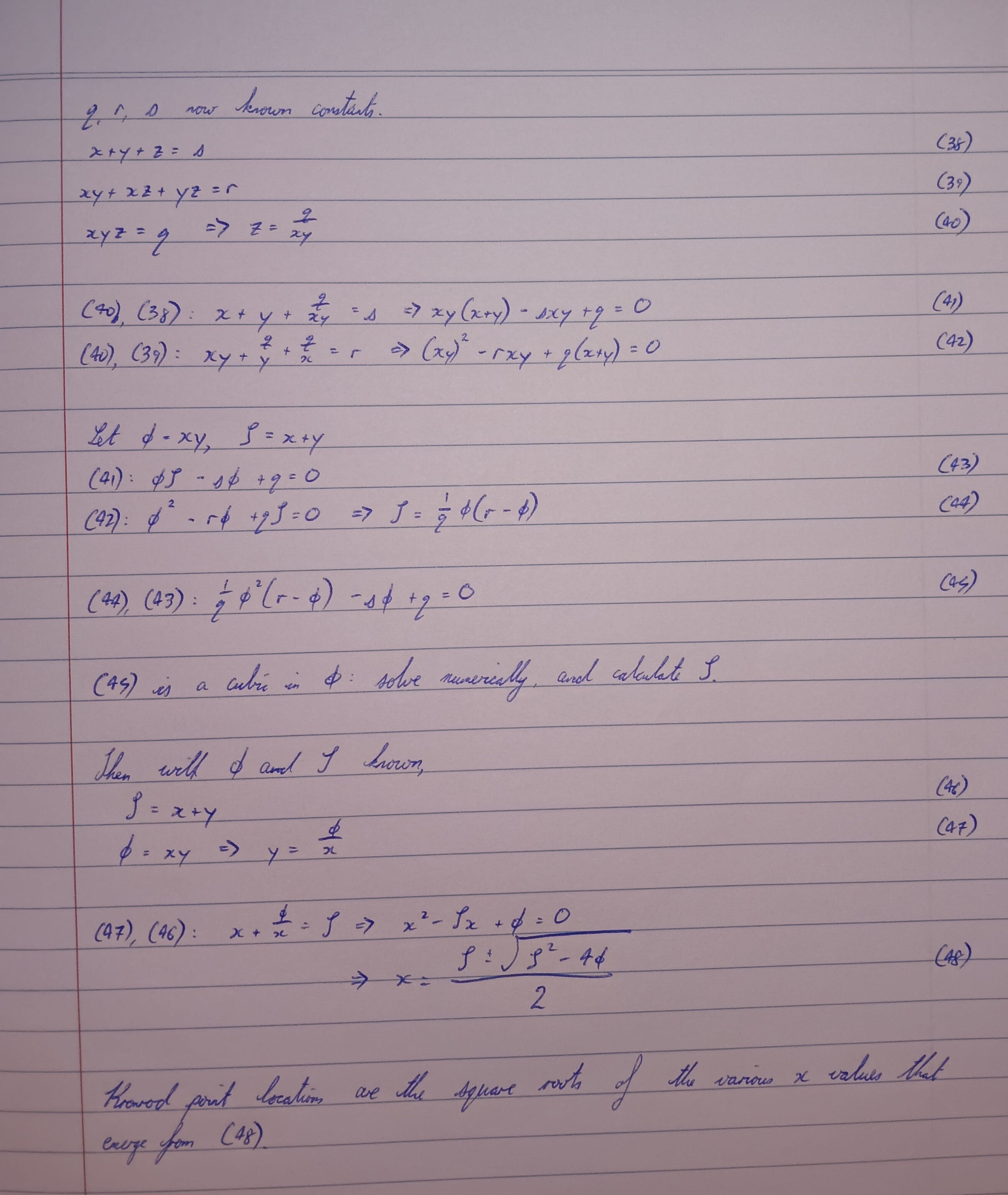
Once the quartic is numerically solved, the four sum-and-product values lead to a cubic equation in xy, and then the procedure is similar to the Gauss N = 6 or 7, with the cubic’s solutions leading to quadratics in x.
Here is some Python code that follows my handwritten work to derive the weights and positions for G7, K15. It’s presented in lines of at most 32 characters to try to make them fit on the telephone screen that you’re probably reading this on.
# Derivation of Gauss-Kronrod
# weights and nodes, starting
# from the Gauss nodes.

import numpy as np

# Known Gauss points
g1_r = 0.405845151377397
g2_r = 0.741531185599394
g3_r = 0.949107912342759

g1 = g1_r**2
g2 = g2_r**2
g3 = g3_r**2

def gamma1(n):
  return (
    1/(2*n+1) - g1/(2*n-1)
  )

def gamma2(n):
  return (
    1/(2*n+1) - g1**2/(2*n-3)
  )

def gamma3(n):
  return (
    1/(2*n+1) - g1**3/(2*n-5)
  )

def alpha(i):
  return (g2**i - g1**i) / g2**i

def beta(i):
  return (g3**i - g1**i) / g3**i

alpha_31 = alpha(3) / alpha(1)
alpha_32 = alpha(3) / alpha(2)

beta_23 = beta(2) / beta(3)
beta_13 = beta(1) / beta(3)

delta = (
  (1 - alpha_32*beta_23) /
  (1 - alpha_31*beta_13)
)

def R(n):
  return (
    gamma3(n)*(1 - delta)
    - alpha_32*gamma2(n)
    + alpha_31*delta*gamma1(n)
  )

# Set up and solve linear system
# for variables
# u = x + y + z + t,
# v = xy+xz+xt+yz+yt+zt,
# w = xyz + xyt + xzt + yzt,
# p = xyzt.

A = np.array([
  [R(7),  -R(6), R(5), -R(4)],
  [R(8),  -R(7), R(6), -R(5)],
  [R(9),  -R(8), R(7), -R(6)],
  [R(10), -R(9), R(8), -R(7)]
])

b = np.array([
  R(8), R(9), R(10), R(11)
])

u, v, w, p = np.linalg.solve(
  A, b
)

def solve(fn, deriv, x):
  # A little solver (not robust)
  # for an equation in one
  # variable,
  # fn(x) = 0.
  #
  # x is a discretisation of the
  # interval to search.

  y = fn(x)
  # First get approximate
  # solutions by looking for
  # sign changes

  sign_change = np.where(
    y[:-1] * y[1:] < 0
  )[0]

  x_init = x[sign_change]

  # Use these as initial
  # guesses for some Newton-
  # Raphson.

  x_soln = []
  for x in x_init:
    for i in range(10):
      x -= fn(x) / deriv(x)
    x_soln.append(x)

  return x_soln

# Setup equations for
# q = xyz,
# r = xy + xz + yz,
# s = x + y + z.

def quartic(q):
  return (
    q**4 / p**2
    - w*q**3 / p**2
    + v*q**2 / p
    - u*q
    + p
  )

def quartic_deriv(q):
  return (
    4*q**3 / p**2
    - 3*w*q**2 / p**2
    + 2*v*q / p
    - u
  )

# Setup equations for
# phi = xy,
# zeta = x + y.
# q, r, s will be defined in
# the main scope.

def cubic(phi):
  return (
    phi**3 / q
    - r * phi**2 / q
    + s * phi
    - q
  )

def cubic_deriv(phi):
  return (
    3 * phi**2 / q
    - 2 * r * phi / q
    + s
  )

N = 1000
interval_disc = np.linspace(
  0., 1., num=N
)

q_soln = solve(
  quartic,
  quartic_deriv,
  interval_disc
)

r_soln = []
s_soln = []
for q in q_soln:
  s_soln.append(
    (v*q - q**2*(w-q)/p)/p
  )

  r_soln.append(
    q*(w - q) / p
  )

# Looping through all (q,r,s)
# combinations leads to the
# same positions being found
# many times each, with
# slight differences due to
# accumulated round-off errors.
#
# I'll average the positions
# by using their rounded values
# as keys to a dict.

x_soln = {}

for q, r, s in zip(
    q_soln, r_soln, s_soln
  ):
    phi_soln = solve(
      cubic,
      cubic_deriv,
      interval_disc
    )

    for phi in phi_soln:
      zeta = (r*phi - phi**2)/q
      Delta = zeta**2 - 4*phi
      x1 = 0.5*(
        zeta + np.sqrt(Delta))

      x2 = 0.5*(
        zeta - np.sqrt(Delta)
      )

      for x in (x1, x2):
        rx = np.round(x, 5)
        if rx not in x_soln:
          x_soln[rx] = []
        x_soln[rx].append(x)

x_final = []

for rx in sorted(x_soln.keys()):
  x_final.append(
    np.mean(x_soln[rx])
  )

# Reverse order for printing:
x_final.sort(reverse=True)

# And finally we solve for the
# weights.  We'll need seven
# equations out of the eleven.

arr = np.array(
  [g1, g2, g3] + x_final
)

base_arr = np.copy(arr)

A = np.zeros((7, 7))
for i in range(7):
  A[i,:] = arr
  arr *= base_arr

b = np.array([
  1/3,1/5,1/7,1/9,1/11,1/13,1/15
])

w = np.linalg.solve(A, b)
w_zero = 2 - 2*np.sum(w)

wg = [w[2], w[1], w[0], w_zero]
wk = [w[3], w[4], w[5], w[6]]

xg = [g3_r, g2_r, g1_r, 0.]
xk = np.sqrt(x_final)

print()
print(
  f"{' Points':<13} Weights")


for i in range(4):
  print(
    f"±{xk[i]:.10f} "
    f"{wk[i]:.10f} "
    "Kronrod"
  )

  pm = " " if i == 3 else "±"
  print(
    f"{pm}{xg[i]:.10f} "
    f"{wg[i]:.10f} "
    "Gauss"
  )
Just imagine how much prettier Substack would be if its code blocks had syntax highlighting.
Here is a comparison between Wikipedia (left) and the output from my Python script (right):
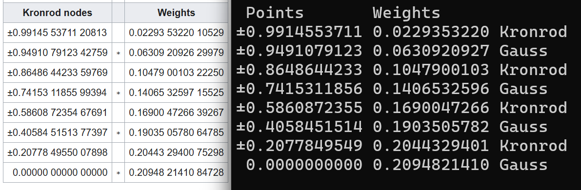
My errors start around the tenth digit.
If you use scipy.integrate.quad on a finite interval, then it’ll be using a G10, K21 integrator. To be honest, if I had to compute the weights and abscissae for such a large system, then I would learn was a Stieltjes polynomial is.
Python code for adaptive integration using G7, K15:
# Adaptive quadrature,
# Gauss-Kronrod G7 K15

import numpy as np

# Gauss-7 node positions
gx = np.array([
  +0.,
  -0.4058451513773972,
  +0.4058451513773972,
  -0.7415311855993945,
  +0.7415311855993945,
  -0.9491079123427585,
  +0.9491079123427585
])

# Gauss-7 weights
gw = np.array([
  0.4179591836734694,
  0.3818300505051189,
  0.3818300505051189,
  0.2797053914892766,
  0.2797053914892766,
  0.1294849661688697,
  0.1294849661688697
])

# Kronrod-15 weights at
# Gauss-7 positions
kw1 = np.array([
  0.209482141084728,
  0.190350578064785,
  0.190350578064785,
  0.140653259715525,
  0.140653259715525,
  0.063092092629979,
  0.063092092629979
])

# Kronrod-15 positions
kx = np.array([
  -0.207784955007898,
  +0.207784955007898,
  -0.586087235467691,
  +0.586087235467691,
  -0.864864423359769,
  +0.864864423359769,
  -0.991455371120813,
  +0.991455371120813
])

# Kronrod-15 weights at
# Kronrod-15 positions
kw2 = np.array([
  0.204432940075298,
  0.204432940075298,
  0.169004726639267,
  0.169004726639267,
  0.104790010322250,
  0.104790010322250,
  0.022935322010529,
  0.022935322010529
])

def scale_points(a, b, x):
  # scale from [-1, 1] to [a, b]
  return (
    a + (b - a)*(0.5*(x + 1))
  )

def gk_quad(a, b, f):
  # Function evaluations at
  # Gauss and Kronrod points:
  fg = f(scale_points(a,b,gx))
  fk = f(scale_points(a,b,kx))

  factor = (b - a) / 2.
  # Gauss-estimated integral:
  int_g = np.sum(gw*fg)*factor

  # Kronrod-estimated integral:
  int_k = (
    np.sum(kw1*fg)
    + np.sum(kw2*fk)
  )*factor

  error = np.abs(int_k - int_g)
  return int_k, error


def adaptive(a, b, f, tol):
  integral, error = gk_quad(
    a, b, f
  )

  if error < tol:
    return integral, error

  intervals = [{
    "lower": a,
    "upper": b,
    "integ": integral,
    "error": error,
    "active": True,
  }]

  for _ in range(100):
    i = np.argmax([
      iv["error"]*iv["active"]
      for iv in intervals
    ])

    a1 = intervals[i]["lower"]
    b2 = intervals[i]["upper"]
    midpt = 0.5*(a1 + b2)

    integ1, err1 = gk_quad(
      a1, midpt, f
    )

    integ2, err2 = gk_quad(
      midpt, b2, f
    )

    intervals.append({
      "lower": a1,
      "upper": midpt,
      "integ": integ1,
      "error": err1,
      "active": True
    })

    intervals.append({
      "lower": midpt,
      "upper": b2,
      "integ": integ2,
      "error": err2,
      "active": True
    })

    old_integ = (
      intervals[i]["integ"]
    )

    old_error = (
      intervals[i]["error"]
    )

    integral -= old_integ
    integral += integ1 + integ2

    error -= old_error
    error += err1 + err2

    intervals[i]["active"] = (
      False
    )

    if error < tol:
      break

  return integral, error

integral, error = adaptive(
  0, np.pi,
  lambda x : np.sin(x**3),
  tol = 1e-4
)

print(integral)
print(error)
The sine wave used in my earlier examples will hardly test an adaptive quadrature algorithm, so instead I will use sin(x^3), integrating from x = 0 to x = tau/2. Here is a representation of the calculation done by the script above:
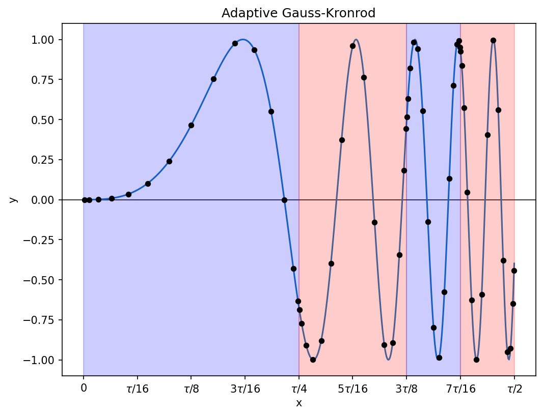
As expected, the sub-intervals are divided more aggressively when the function oscillates more rapidly. A total of 105 function evaluations were needed here, 15 for each of 7 sub-intervals integrated (four of these survived to the end of the calculation, three were replaced by finer sub-intervals).
The true value of the integral, as provided by Wolfram Alpha, is approximately 0.41583381465627398042. The Gauss-Kronrod calculation above is off by about 1e-12.8 For comparison, here are the errors for the other methods in this post, for a slightly larger number of function evaluations (I’ve used a target of 120 evaluations so that I can at least approximately reach it with an integer number of sub-intervals for all the Gauss rules: Gauss-2 uses 60 sub-intervals, Gauss-3 uses 40, etc.):
Method      #evals  Error
Rectangular  120   -7.89e-04
Trapezium    120    1.59e-03
Simpson's    119   -6.93e-05
Gauss-2      120    4.33e-05
Gauss-3      120   -2.55e-06
Gauss-4      120    1.33e-07
Gauss-5      120   -1.30e-09
Gauss-6      120   -1.12e-09
Gauss-7      119    1.69e-10
This looks superficially like an excellent demonstration of the greater efficiency of adaptive quadrature, since all the non-adaptive errors in the table are orders of magnitude greater. But I used a 15-point Kronrod rule for the adaptive calculation, and a hardened sceptic may point out that a 15-point Gauss rule with 75 function calls calculates this integral to within 4e-14. Perhaps a pure-Gauss adaptive scheme, “G7 G15”, might therefore be more efficient than Gauss-Kronrod here?
The answer is no: while the eventual error is indeed lower (5e-15), the same subdivisions of the interval would take place, leading to 22 × 7 = 154 function calls as opposed to 15 × 7 = 105. And a “G5 G10” adaptive scheme, which uses the same number of function calls per sub-interval as G7 K15, requires analysing 13 sub-intervals instead of 7 to get the estimated error below the tolerance (the Gauss-5 is too inaccurate).
Unless you know in advance what sub-intervals you need, this example of integrating sin(x^3) is evidence that the QUADPACK people are correct to use Gauss-Kronrod, which is a happy conclusion for me. I would not expect to overturn such a well-established library.
Browsing the results table, I find it remarkable how much improvement there is in increasing the number of points in the Gauss rule. The error reduces by about an order of magnitude per Gauss point, for the same number of function evaluations! It is a lot of orders of magnitude.
3. Coronidis loco, an empty final section
Integrating sin(x) will be an implicit exercise.
Substack Latex doesn’t do equation numbering and cross-referencing, but you can \tag{} an equation with a manually-entered label.
I used Legendre polynomials.
I haven’t studied Runge’s phenomenon.
Gauss integrates from 0 to 1 rather than from −1 to 1, so a simple ctrl-F for digits from modern tables wouldn’t find any matches even if the Wikisource link didn’t put Gauss’s tables in images. I haven’t tried studying Gauss’s calculation methods, which are different from mine.
It’s almost tempting to give the manual calculation a try. Since we expect each root of the cubic to be between 0 and 1, fifty bisections will find one to within 1e-15; Newton-Raphson might get the digits faster once close, though I’m not sure how slow the necessary long division at each step would be.
It looks daunting at first glance to have to cube numbers up to 15 digits long repeatedly, but it will often only be necessary to do more manageable updates from an earlier calculation. e.g. you could store the square and cube of 0.1234567 after you calculate it for the first time, so that when you need to cube 0.12345673 and 0.12345679, you have most of it already done. You also wouldn’t need to keep track of all the less-significant digits.
This was a feature of some of my undergrad work. An abstract algebra exam question would be written with the intention of testing if the student could recall and apply some theorem which led to a quick solution, but the numbers involved might be small enough to brute-force it. I recall a third-year exam which had a question where you needed to solve
and I just squared every number between 1 and 43 and divided by 85 to get the remainder.
Then in a fourth-year exam – my memory is fuzzier here, so I will make up some plausible details – I reached an expression involving a product of 11 terms, each term being x minus an 11th root of unity. Instead of recognising the cyclotomic polynomial, I expanded the 11-term product and simplified manually. “You were the one who did those horrendous calculations,” the lecturer said to me after he’d marked the exams, but my horrendous calculations were not wrong.
This skill is very useful for taking exams after not studying hard enough, and not very useful for anything else.
Someone paying close attention may notice that I asked for a rather loose tolerance of 1e-4 in my Python code, and yet I got a result that was extremely close to the true value. Once the interval has been subdivided enough, the estimated error becomes close to the actual error for the Gauss-7 calculation. So we get a Gauss-7 calculation that is within 1e-4, and then 8 extra points are used for every sub-interval in the Kronrod-15 calculation, driving the actual error much lower.
i havent finished this and maybe i never will but i enjoyed what i read so far and need to ask: why do you think the trapezoidal approximation (the second thing you showed) doesn't improve much over the rectangle? initially, i thought "aha this is an example of taxicab metric behaviour" but it clearly isnt, we're going along slanted lines now, and anyway smaller rectangles is better (right?) so it cant be like taxicab at all...