


I have opinions about the nine definitions of a sample quantile
Hazen 4 lyf

My title is facetious: there are an infinite number of possible definitions of a sample quantile. When you ask your favourite statistical package for a quantile of some data, what calculation should it do?
It may seem strange that there’s anything to debate here. We learn in high school that the median is the middle value of a sorted set, or the average of the two middle values if the sample size is even. Other quantiles should be similar, just counting elements as needed.
But perhaps I can make you hesitate a little. Given a set of four values {10, 15, 30, 40}, my intuition leaps to the idea that the four values correspond to the quantile levels of 25%, 50%, 75%, and 100%. I immediately correct myself: the median – quantile level 50% – should be the average of 15 and 30, not 15 on its own. Reasoning similarly, the 25% mark should be the average of 10 and 15, and the 75% the average of 30 and 40.
(For clarity, I will do my best to explicitly distinguish between quantile levels and quantile values. The median of the set {4, 6, 8, 12, 20} is 8; for a quantile level of 0.5, the quantile value is 8. Quantile levels exist on an axis between 0 and 1, which I sometimes refer to as a probability axis.)
On the other hand, if Alice scored 10 points, Bob scored 15, Charlie scored 30, and Diane scored 40, then we could reasonably say that Alice scored in the 25th percentile (and also in the 1st percentile, 2nd percentile, etc.), Bob scored in the 50th percentile (and in the 26th percentile, etc.), Charlie scored in the 75th percentile, and Diane scored in the 100th, or top, percentile. The “1st percentile” is that part of the probability axis between 0 and 1%, the “25th percentile” is between 24% and 25%, and Alice comprises 25% of the dataset, covering both of these percentiles.
So we already have two competing, related concepts, using two words, quantile and percentile, that might not always be perfectly interchangeable.
One issue with the second definition is that we are effectively counting percentiles from 1 to 100. But a probability axis ranges from 0 to 100%, and in a quantile calculation we have to specify a quantile level, or cumulative probability, which is defined on the full interval from 0. A definition motivated by a 1-100 range will therefore be asymmetric. In the context of a statistical calculation, I think such definitions are bad, but we will nevertheless see a couple like this below, in amongst more symmetric offerings.
The standard reference on the subject is Hyndman and Fan (1996), which describes nine competing definitions of a sample quantile, many being supported by at least one statistical package in common use at the time. Those authors were hoping to encourage standardisation on their preferred choice, but instead their full set of nine has become quasi-canonical, with both R and NumPy supporting all of them.
How much of a difference does any of this make? For large datasets, the answer is usually “not much”. For small datasets, it’s more interesting. I generated 100 random numbers from a standard normal distribution, and calculated the quantile values at levels 0.05 and 0.95 with each of the nine methods.
     Quantile_level
Defn   0.05   0.95
------------------
R-1  -1.425  1.686
R-2  -1.398  1.709
R-3  -1.425  1.686
R-4  -1.425  1.686
R-5  -1.398  1.709
R-6  -1.423  1.730
R-7  -1.372  1.689
R-8  -1.406  1.716
R-9  -1.404  1.714
Output values varied from -1.372 to -1.425 in the lower tail, and from 1.686 to 1.730 in the upper tail. A few percent. Sometimes the differences are larger, sometimes smaller; for a set of size 100, it depends on how different the random number generator’s fifth and sixth smallest or largest values are.
(The theoretical quantile values in this case are approximately ±1.645. So we should note in passing, and commit to long-term memory, that if you have to estimate these quantiles with a sample size of only 100, then you have bigger problems than the choice of definition. Still, it’s annoying to have even more uncertainty introduced by the fact that you’ll get different answers with the default settings of Excel, R, Stata, MATLAB, etc.)
Following Wikipedia, the definitions in this post are labelled R-1, R-2, etc., the number being the corresponding type parameter of R’s quantile function; this numbering matches the order in the Hyndman and Fan paper.1 In each section header below, the string that follows the R number ("inverted_cdf" etc.) is the value of the corresponding method argument of numpy.quantile, this argument having been introduced in NumPy version 1.22, Python 3.8.
For each definition, I show a graph of the quantile value against the quantile level for the four-element dataset {10, 15, 30, 40} and make some comments. For definitions that involve linear interpolation between sample values, I also study the overall bias as a function of the quantile level.
Python code for the bias graphs is available on GitHub.
Discontinuous definitions
The first three definitions always return one of the values in the dataset, or an average between two of them.
R-1, "inverted_cdf"

Each sample occupies a fraction 1/N of the quantile level axis. For a quantile level exactly in between two samples, it chooses the lower value. Since this definition doesn’t average between two samples – e.g. the median of an even-sized data set will be the lower of the two middle values – it’s an inferior version of R-2.
R-1 is used by Wolfram’s Quantile.
R-2, "averaged_inverted_cdf"

The same as R-1, but averaging when you’re half-way between two values. If you’re going to use one of the discontinuous definitions, this is the one to use.
R-2 is the default option for Stata’s pctile and SAS’s PROC UNIVARIATE.
R-3, "closest_observation"

For a given quantile level p, let k be the closest integer in {1, …, N} to N*p, rounding .5 to even. The quantile value is the k-th smallest sample value.
This definition is an asymmetric abomination. The minimum value takes up an extra half-sample’s worth of the probability axis, at the expense of the maximum. The round-to-even at the discontinuities is comical, like they’re trying to make their systematic off-by-half error unbiased.
Intellectual honesty requires me to try to get inside the head of whoever came up with this monstrosity. I’ve tried! I can’t think of how this definition can be justified even by accident. Some historical possibilities:
Someone went “k equals N times p rounded” and either didn’t notice or didn’t care that N*p is on a scale of 0 to N, while k is on a scale of 1 to N.
Someone went, “You know how Alice scored at the 25th percentile and Bob at the 50th? Probably with a bigger sample size, the 26th percentile would be closer to Alice’s score than to Bob’s, and the same goes for all quantile levels up to half-way between them.” This is, I think, the most superficially persuasive argument for R-3, though it doesn’t work on its own terms because Bob scored in the 26th percentile as well as in the 50th.
???
R’s help describes R-3 as the “SAS default till ca. 2010”, but I think this is incorrect and unfairly maligns SAS. Perhaps SAS was the first statistical software to introduce the R-3 definition, but any such crime must be ancient history: the earliest documentation I could find was from 1992, in the 3rd edition of the SAS Procedures Guide, version 6, and R-2 (PCTLDEF=5) was the default even then.
Continuous definitions
All subsequent definitions involve linearly interpolating between sample values; the question is where to plot each point on the quantile level axis. Let p(k) be the quantile level for the k-th smallest value (the “k-th order statistic”). This family of definitions all use a linear relation between k and p(k), i.e. p(k) = c1*k + c2 for some constants c1 and c2.
The coefficient c1 will be somewhere near 1/N, since we need to place N points in between somewhere near 0 and somewhere near 1. By convention (followed by SciPy and Julia), parameters α and β are introduced as an offset from N + 1 in the denominator:
For symmetry, we require that p(k) = 1 - p(N - k + 1), which implies α = β and therefore a functional form of
One consideration is that a piecewise-linear curve can be a very poor approximation to the true distribution, most notably in the case of heavy tails. Consider a Pareto distribution with probability density function 2/x^3 for x in the domain [1, ∞). Its quantile function, or inverse cumulative distribution function, looks like this:
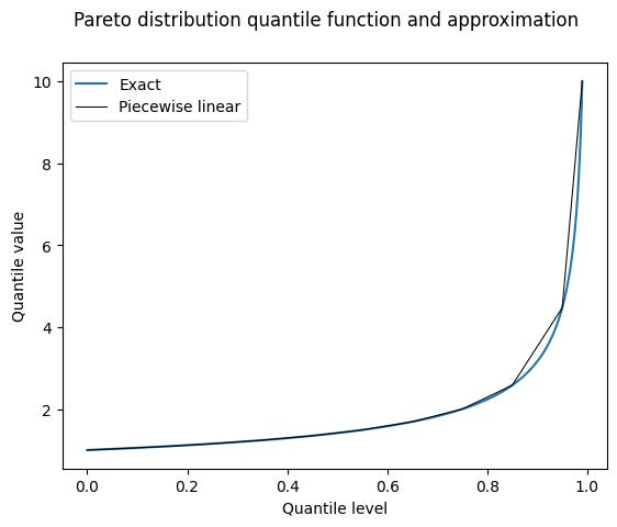
Even if the sample quantile points are plotted at exactly the correct quantile levels and values (miraculous), the linear segments will systematically lead to overestimates in between them, since the true quantile function is concave upward.2 Having more points in the curve – i.e. a larger sample size – will reduce the errors, but the systematic bias is inherent to the method.
The best we might hope for is that the points are plotted at the wrong quantile levels, and we get some partially offsetting errors. But really, I think that if it is important to estimate quantile values from samples coming from a distribution like this, then it is best to use a fancier technique than the default quantile function offered by your favourite statistical package.
Even in the much more gentle normal distribution, the curvy nature of the inverse CDF curve means that the linear interpolations can lead to systematic errors, which are most visible in the tails. The discussion of R-9 below covers this case in more detail.
When a set of random numbers is drawn from a known continuous probability distribution, it is possible to numerically compute the expectation of the sample quantiles for each definition.3 The known distribution also gives the true quantile values, and this allows the bias (expectation minus true) for each definition to be calculated at each quantile level, for a given sample size.
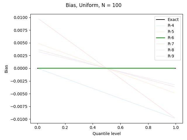
I’ve done this for the uniform distribution on [0, 1), the standard normal distribution, and the Pareto distribution shown above, for each of the definitions based on linear interpolation, using N = 100. All graphs show quantile levels between 0.01 and 0.99. Here are the results for the uniform distribution (which could be computed exactly, rather than using numerics):

We will see below that R-6 is constructed to be unbiased for the uniform distribution.
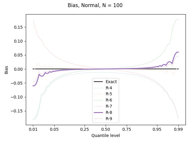
For the other two distributions, I’ll use a nonlinear horizontal axis to better show what happens in the tails, where most of the action is. Here are the results for the standard normal distribution:

The sharp points in the curves are where the sample values are being plotted; the curvy arcs connecting them correspond to the linear interpolations, which are warped by both the nonlinear behaviour of the true quantile values, and my nonlinear axis.
Since the 0.95 quantile level has a value of about 1.645, and the biggest biases there are almost 0.05 in magnitude, a poor choice of definition could lead to a systematic bias of about 3% – with much variability from dataset to dataset!
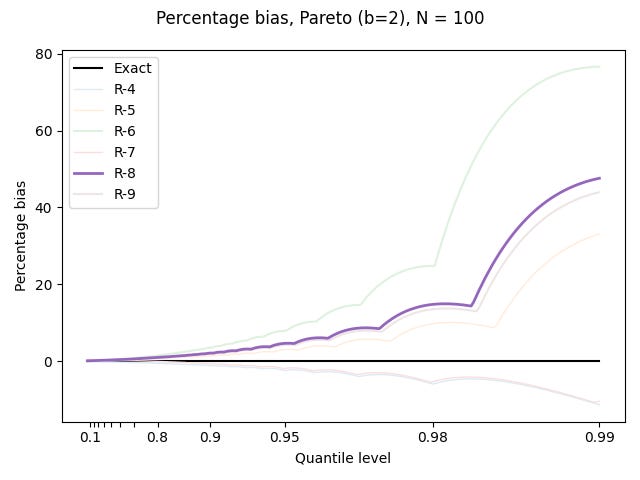
For the Pareto distribution, I plot the bias as a percentage of the true value:

Things are pretty bad out in the tail.
R-4, "interpolated_inverted_cdf", (α, β) = (0, 1)

The asymmetry of R-3 is still abominable in continuous form. Again there is a superficially appealing argument for it if you want to consider the upper bound of a percentile: we linearly interpolate between Alice’s score at the 25th percentile and Bob’s score at the 50th. But again it doesn’t work: if we had a larger sample size, then Alice and Bob would tend to find themselves at lower percentiles than their current upper bounds. R-4 systematically underestimates the quantile values, and thankfully all remaining definitions are symmetric.
Bias curves for the uniform, normal, and Pareto distributions:


R-5, "hazen", α = 1/2

Hazen in his 1914 paper, “Storage to be provided in impounding reservoirs for municipal water supply” (Transactions of the American Society for Civil Engineers, 77, 1539):
That is to say, if there are 50 terms in the series, each is taken to represent 2% of the whole space. The first term will be plotted at the middle of the first 2% strip; that is, on the 1% line; the second term will be plotted in the middle of the second strip, or on the 3% line, etc.
Early in my sample quantile journey, before I learned about all these definitions, I had seen different programs output the R-2 and R-7 definitions, and someone’s Excel spreadsheet accidentally implement R-3. I got out a pen and paper and tried to figure out how I would define a sample quantile, and I came up with Hazen’s approach. It’s simple, intuitive, and (happily) it gives good results, especially for the normal distribution.


Well, none of these definitions are good with the Pareto distribution, but R-5 at least overestimates by less than the other overestimating definitions.
If it were up to me, R-5 would be the default across statistical packages. Cunnane’s 1978 survey, which ends up recommending none of these nine definitions, says that “Contrary to traditional arguments… the Hazen formula is quite good while the Weibull formula [R-6] is not nearly as good.”
Early in their paper, Hyndman and Fan list six desirable properties for a sample quantile function. In their concluding section, they write that “Only [R-5] satisfies all six properties P1–P6. However,” and then they continue with some egghead nonsense.
R-5 is the default option for MATLAB’s quantile function and EViews’ statistics.
Egghead nonsense definitions
Why would we need anything more complicated than R-5? Hyndman and Fan:
This is an analogous situation to the problem of defining the sample variance. In that case the statistical community has adopted the unbiased definition (with denominator n - 1) as the standard rather than the more intuitive average of squared deviations (with denominator n)….
Regretfully, I acknowledge that this is a fair point. Let’s continue.
R-6, "weibull", α = 0

Suppose we have a sample size of 2. The R-5 definition would tell us to plot the minimum value at a quantile level of 0.25, and the maximum at a quantile level of 0.75.
But now suppose that we’re drawing from a uniform distribution on [0, 1]. What is the expectation of the minimum of two independent random numbers from this distribution? Let the first random number be x. With probability (1 - x), this first number is the minimum. With probability x, the other random number is the minimum. In the latter case, its conditional expectation is x/2 (since it’s uniformly random and less than x).
Conditional on the first random number being x, the expectation of the minimum is therefore x(1 - x) + x^2 / 2 = x - x^2 / 2. Integrating over x from 0 to 1 gives the overall expectation of the minimum of 1/3; by symmetry, the expectation of the maximum is 2/3.
Therefore, the argument goes, instead of plotting the two values at the R-5 quantile levels of 1/4 and 3/4, we should plot them at 1/3 and 2/3.
The idea generalises. Given N independent random numbers uniform on [0, 1], the expectation of the k-th order statistic is4 k/(N + 1). By plotting sample values at these quantile levels, we get results that are unbiased for the uniform distribution.
But we get the worst overestimates of the variability for the normal and Pareto distributions:


R-6 is used by Excel’s PERCENTILE.EXC, and is the default option of gretl’s quantile, SPSS’s PERCENTILES, and Python’s statistics.quantiles.
R-7, "linear", α = 1

It was bad when R-4 plotted a point at a quantile level of 1, and here it’s bad at both ends, with a point plotted at quantile level 0 as well.
The Wikipedia table describes this definition as “Linear interpolation of the modes for the order statistics for the uniform distribution on [0,1].”5 This struck me as a very peculiar motivation (who uses modes?). But I dutifully checked Hyndman and Fan, who write that “Gumbel (1939) also considered the modal position…”.
And it’s true, Gumbel did consider the mode (reference, Comptes rendus de l'Académie des sciences, 209, 645), before immediately saying that the mean position (R-6) is preferable, because when using the mean, the minimum and maximum will be assigned probabilities that differ from 0 and 1. I agree with Gumbel that R-6 is better than R-7 for exactly the reason he gives.
But I suspect that these points are of historical interest only. When R-7 is the default option for a quantile function, what I reckon happened – just based on me trying to get my head into all these definitions – is that someone went:
the minimum should be at 0;
the maximum should be at 1;
linearly step between them.
Or they were copying what some other language does.
I don’t think there was much more thought put into it; no-one was picturing a probability distribution and going, “This is a situation that really calls for the mode.” It’s just a coincidence that R-7 can be derived from modes of the uniform distribution’s order statistics, allowing it to be grouped with R-6 (means) and R-8 (medians).
It’s a garbage definition which systematically understates the variability: you will usually have more variability in the full population than in your finite sample, and it’s silly to implicitly assume that your sample extremes are equal to the population extremes. If you’re trying to estimate risk based on some sample quantiles, then this definition will lead to false over-confidence.


The best that can be said about it is that the percentage underestimates for the Pareto distribution are not as large as the percentage overestimates by the other symmetric definitions.
R-7 is used by Excel’s PERCENTILE.INC, and is the default definition for R’s quantile, Julia’s quantile, and numpy.quantile.
R-8, "median_unbiased", α = 1/3

Unlike for the mean and mode, it’s either difficult or impossible to get an exact expression for the median of the k-th order statistic of the uniform distribution. But a good approximation is6 (k - 1/3) / (N + 1/3).
If an estimator is median-unbiased, then it’s greater than the true value as often as it’s less. What’s nice in the present context is that median-unbiased for the uniform distribution implies median-unbiased for all continuous distributions: the one-to-one mapping between two distributions will map quantiles to quantiles.
Since it’s impossible to choose a definition that’s mean-unbiased for all distributions – as we’ve seen, what’s right for the uniform distribution is wrong for the normal distribution – median-unbiasedness becomes an attractive alternative goal; the definition has an objective reason for being. I still care about means, and therefore prefer R-5, but tastes may vary. First let’s look at the mean-bias graphs as shown for the earlier definitions.

It’s clearly one of the better definitions for the normal distribution, even on my preferred teams (mean bias). How does it do on median bias? Since we don’t have exact values to work with, I made 100,000 sets of 100 random numbers, and for each quantile level, calculated the fraction of values that were above the true value (for the uniform distribution). Here are all the definitions in full colour:

And here is R-8 highlighted:

Pretty much bang on, unless you’re so far into the tails that you’re estimating from the minimum or maximum. I had some concern that the linear interpolations could lead to more median bias for other distributions, but the changes were small enough not to bother showing.
My preferred R-5 is far from the worst by the median-unbiasedness measure, much as R-8 is decently competitive on mean-unbiasedness for the normal distribution.
R-8 was the recommendation of Hyndman and Fan, and it has become the default option of Maple’s Quantile.
R-9, "normal_unbiased", α = 3/8
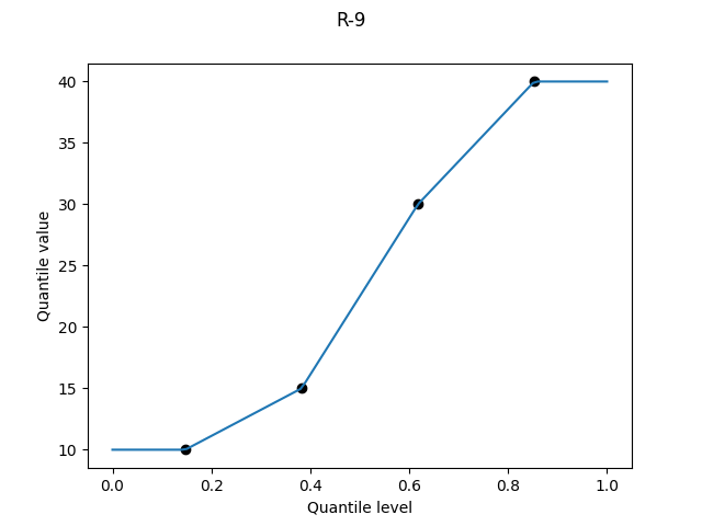
This definition is an unfortunate historical accident. The idea is to choose α so that results match the expectations of the order statistics of the normal distribution. It’s a noble goal, since the normal distribution is encountered far more often than the uniform distribution, for which we have R-6.
But the normal distribution is not so kind. The “constant” α should vary with both the sample size N and the order k. Blom in 1958 (Statistical Estimates and Transformed Beta-Variables, p70) calculated some α values for N up to 20, finding them all between 0.33 and 0.39, and suggested 3/8 as a decent approximation. He was aware that α may grow larger for larger N, not ruling out values up to 1/2 in the limit.
If it were up to me, R-9 wouldn’t exist. That “Blom’s approximation” of α = 3/8 became widely cited is a sociological phenomenon rather than because it’s an objectively optimal constant which different people would independently converge on. Already by 1961, in a paper I found only after I’d made my own efforts described below, Harter had already calculated more precise approximations than Blom’s (and indeed than mine).
To try to derive some numbers for myself, I did the following for some different sample sizes N:
Compute the expectations of all order statistics X_(k).
Convert the expectations of the order statistics to probabilities p_(k) by applying the standard normal CDF.
Regress p_(k) against k, fixing the constant term so that the regression is symmetric either side of (p = 1/2, k = (N + 1)/2).
The reasoning behind this procedure may seem obvious to some readers, but is not well internalised in my head, so I will spell it out. Let G(x) be the CDF of the standard normal distribution. If the above regression is perfect, then p_(k) = G[E(X_(k))] for all k, or
Meanwhile, let Q(p) be the sample quantile function for a quantile level p. At the plotting position p_(k), the expectation of Q(p_(k)) is
exactly as desired to make the sample quantile function unbiased: the expectation of the sample quantile function at p_(k) is equal to the theoretical quantile function at p_(k).
(Fun fact: I spent hours in conceptual confusion before reaching the above procedure. When working with the uniform distribution, both the values and the quantile levels are defined over the same unit interval, and you can allow yourself not to think too carefully about it: everything just works. With the normal distribution, the values are on a different scale. I ultimately want a regression model for a probability axis, and how do I regress with normally distributed values?
My first approach was to do Monte Carlo, generating for each trial a sample of N standard normal random numbers, sorting them, applying the standard normal CDF to them to get onto (0, 1), and averaging these values to get approximate mean order statistics. It was only when I ironed out all my bugs and saw a result almost identical to R-6 that I realised that I had applied the CDF too early, and that I was calculating expectations of order statistics for the uniform distribution.)
Here are my results:7
   N   alpha  R-squared
   2  0.3301  1.000000000
   5  0.3541  0.999996227
  10  0.3713  0.999997922
  20  0.3854  0.999999503
  50  0.3982  0.999999933
 100  0.4043  0.999999977
1000  0.4120  0.999999999
Harter notes that you can get more precision by using one alpha value for the minimum and maximum, and a second alpha value for all other order statistics.
Let’s first see the results for α = 3/8.


A surprising observation is that R-9 is not obviously better than R-5 for the normal distribution. To make what’s happening clearer, I’ll throw away all the other definitions, and also introduce a misnamed “R-10”, defined with α = 0.4, which according to my regressions should be better for my N = 100 sample size.

The sharp points in the curves are the sample values, and we can see that for “R-10” especially, these points are plotted with less bias than is shown by R-5. However, the linear interpolations between these points make the bias worse for R-9 and “R-10” but better for R-5 – the latter is benefiting from some partially offsetting errors.
Things would have looked incredibly good for R-5 if I had shown only only the quantile level of 0.05 (or 0.95): there the corresponding k value is (N + 1 - 2α)*p + α = 5.5, requiring an interpolation to half-way in between two values, near a local minimum of the bias from this definition. R-5 would still lose to the definitions that specifically target the normal distribution, but not by much: a bias of +0.34% for R-5, versus -0.32% for R-9 and -0.18% for “R-10”.
That particular set of parameters (N = 100, p = 0.05) is a case of relevance to me in my day job, but the details of how these definitions perform will vary with the sample size and the quantile levels of interest.
If you want more amateur spitballing about normal distribution order statistics, then I recommend Gwern’s post on the subject, which has a collection of references that was useful to me.
By coincidence – the doc cites Cunnane, who was compromising between various cases – the scipy.stats.mstats.mquantiles default is α = 0.4, which serves as a good value for the normal distribution across many sample sizes.
Conclusions
I like the Hazen definition, R
type=5. Don’t overthink it.You’ll get horrific biases when estimating quantiles in a heavy tail by one of these simple methods. I assume there’s a vast literature covering more sophisticated techniques, but I am unfamiliar with it; this post represents the state of my knowledge at the time of writing.
I have focused almost exclusively on the overall bias of each sample quantile definition, and almost totally ignored the uncertainty inherent in estimating quantiles near the extremes from small samples. The latter is usually more important than which definition you use.
You better believe I have to check Wikipedia every time to re-learn which way a convex function curves.
In a fit of laziness, I used the formulation on this page rather than deriving it myself, but don’t worry, there’ll be some factorials in the next footnote. The integral formula is completely standard anyway, and can presumably be found in many textbooks.
In my first attempt at deriving this result, I started by writing down a formula for the cumulative distribution function, then taking a derivative to get the probability density function. But after seeing the result stated without proof in Gumbel’s 1939 paper, I was inspired to look at the problem again and I saw that the pdf can be derived directly.
We want to find the probability that the k-th order statistic (i.e. the k-th smallest value; k = 1 for the minimum) – is in the interval [x, x + dx]. We get a factor of dx from the probability that one of the N samples lies in this interval, and a factor of N since the k-th smallest may be any of the N. There must be (k - 1) samples below x and (N - k) samples above x + dx; these give factors of x^(k - 1) and (1 - x)^(N - k) respectively. There are (N - 1)-choose-(k - 1) ways to distribute these N - 1 samples above and below the k-th smallest. The pdf f_k(x) is therefore
though the factorials at the start can be tidied a little to give
To find the expectation, we multiply the pdf by x and integrate from 0 to 1:
The integral can be computed by integrating by parts k times, differentiating the x term until it is a constant, and integrating the (1 - x) term. The products at 0 and 1 will all be zero until x^k has been reduced to a constant; the minus sign brought out from (1 - x) will cancel with the minus sign in the integration by parts formula. The derivatives will give factors of k, k - 1, … in the numerator; the integrals will give factors of N - k + 1, N - k + 2, …, N in the denominator. As if by magic, these cancel with the binomial coefficient, leaving
The pdf f_k(x) for the k-th order statistic was derived in the previous footnote. The mode is the maximum; to find it, we take the derivative and set it equal to zero. Applying the product rule gives us
from which we can factor out most terms:
Let’s trust that the mode isn’t at x = 0 or x = 1; the interesting term is the one in square brackets, which leads to the linear equation
or
Integrating the pdf from 0 to some number less than 1 means that terms don’t conveniently vanish during the integration by parts. Hyndman and Fan cite some approximation work; I did some numerical tests that agree closely with the α = 1/3 result.
My tests involved finding the approximate medians of the normal distribution’s order statistics by Monte Carlo, and then doing a linear regression against the order k. But since I want to fix the constant so that I have the appropriate symmetry, I have to be a little careful in setting up the input and output arrays for the call to numpy.linalg.lstsq.
Start with the form
and write it as
We must have c_2 = -α*c_1, and since c_1 = 1/(N + 1 - 2α) and therefore α = (N + 1 - 1/c_1)/2, it follows that
or
This is now in a form ready to be passed to lstsq: a single input array of k - (N+1)/2 (no array of ones for a constant term), and an output array of p - 1/2.
Substack does not support side-scrolling code blocks, so I’ve broken up my python lines into little pieces, in the hope that the drab colourless text may be almost readable on at least one mobile device. If you run this code, and increase N_trials and/or N too much, then you may run out of RAM.
import numpy as np

N_trials = 1000000
N = 100

rng = np.random.default_rng()
x = np.zeros((N_trials, N))

for i in range(N_trials):
  x[i, :] = np.sort(
    rng.random(N))

median_kth = np.quantile(
  x, 0.5, axis = 0)

def lin_reg(input, output):
  # Regression of output against
  # input; input is 1d array.
  N = len(output)
  input = input.reshape((N, 1))
  var_out = np.var(output)
  reg = np.linalg.lstsq(
    input, output, rcond=None
  )

  slope = reg[0][0]

  R_sq = (
    1 - reg[1] / (N * var_out)
  )[0]

  return (slope, R_sq)

# Set up a symmetrised
# linear regression

reg_p = median_kth - 0.5

input = (
  np.arange(1, N + 1) -
  0.5 * (N + 1)
)

m, R2 = lin_reg(input, reg_p)
alpha = 0.5*(N + 1 - 1/m)

print(f"alpha = {alpha:.4f}")
print(f"R-sq  = {R2:.9f}")
For N = 100, I get results like
alpha = 0.3279
R-sq = 0.999999958Python code:
import numpy as np
from scipy.integrate import quad
from scipy.stats import norm

def log_factorial(n):
  return np.sum(
    np.log(
      np.arange(1, n + 1)))

def wrapper(N, k):
  # Returns a function whose
  # integral is the expectation
  # of the order statistic.

  log_factorials = (
    log_factorial(N) -
    log_factorial(k - 1) -
    log_factorial(N - k)
  )

  def integrand(t):
    log1 = norm.logcdf(t)
    log2 = norm.logcdf(-t)
    log3 = norm.logpdf(t)

    return t * np.exp(
      log_factorials +
      (k - 1)*log1 +
      (N - k)*log2 + log3)

  return integrand

def lin_reg(input, output):
  # Regression of output against
  # input; input is 1d array.
  N = len(output)
  input = input.reshape((N, 1))
  var_out = np.var(output)
  reg = np.linalg.lstsq(
    input, output, rcond=None
  )

  slope = reg[0][0]

  R_sq = (
    1 - reg[1] / (N * var_out)
  )[0]

  return (slope, R_sq)

N_samples = [
  2, 5, 10, 20, 50, 100, 1000]

print(f"   N   alpha  R-sq")

for N in N_samples:
  x = np.zeros(N)
  half_N = N // 2

  # Compute expectations of
  # order statistics:
  for k in range(0, half_N):
    x[k], _ = quad(
      wrapper(N, k + 1), -9, 9)
    x[-k - 1] = -x[k]

  p = norm.cdf(x)

  # Set up a symmetrised
  # linear regression
  reg_k = np.arange(1, N + 1)
  reg_p = p - 0.5
  input = reg_k - 0.5*(N + 1)
  m, R2 = lin_reg(input, reg_p)
  alpha = 0.5*(N + 1 - 1/m)

  line = f"{N:4d}"
  line += f"  {alpha:.4f}"
  line += f"  {R2:.9f}"
  print(line)