Measuring pitch

With some success

This post is a DIY Wings of Pegasus YouTube analysis video.¹ After using Demucs to extract a vocal track from a song recording, I have a python script that processes the track and draws a graph of the estimated pitch against time; I’ll just do a few seconds at the start of each song. The pitch detection isn’t perfect, but it’s good enough for me.

First up is Chappell Roan’s ‘Femininomenon’, which my YouTube Recap says was my second-most listened-to song in 2025 (number three was ‘So Am I’ by Ava Max):

My pitch-detection code looks mostly stable, and even in the couple of places it jumps up or down dramatically, I don’t mind it: I can hear a brief flash of a high-pitched sound just after the 4-second mark, and I hear a bit of vocal fry when the pitch graph goes low.

I don’t have the same ear that the Wings of Pegasus guy has, and I can’t honestly rant with feeling about how modern pop music producers ruthlessly remove any emotion conveyed by a voice that’s a little sharp or flat, turning talented singers into soulless machines. But I think that the graph above is consistent with pitch correction having been applied: we see a lot of notes held near perfectly horizontal at the gridlines, which represent standard-tuning note frequencies. The extremely brief (I can’t hear it!) perfect jump from A♭ to B♭ and back just before the 5-second mark looks particularly suspicious.

By contrast, here’s Bruce Springsteen with ‘Sherry Darling’ (1980):

Springsteen’s voice is definitely not being snapped to the standard-tuning frequencies here, often hanging around midway between the gridlines – appropriately loose for a quasi-drunken party song.

My code starts getting the octave wrong in both directions a little before the 5-second mark, and this time I can’t hear a good reason for it. Such errors are not shocking. The voice generates a series of harmonics; the first is at the frequency we perceive as the pitch, and the second is at double the frequency, i.e. an octave higher. If the code “latches onto” the second harmonic, then it will output a pitch that’s up one octave.

My code doesn’t actually go hunting for a frequency, though, it instead tries to find the period of the sound waves. If we shift the waves by one full period, then they will approximately line up with where they were to begin with. But the same is true if we shift by two full periods, and if the code calculates a period that is twice as big as it should be, then the calculated frequency is halved, and the reported pitch goes down an octave.²

In a lower register, here’s Cat Stevens with ‘Father and Son’, his voice often rapidly gliding up and down in a way that I hadn’t appreciated until seeing it plotted (connected dots are 0.02 seconds apart):

I had to manually truncate the vertical axis upper bound, because a couple of times (despite some attempts to filter out such cases) my code found a frequency several octaves higher. There’s also an octave drop right at the end.

One of the most viral Wings of Pegasus videos is on Karen Carpenter’s excellent vocal accuracy in an era before pitch correction. Here’s the opening line of the Carpenters’ ‘I Need to Be In Love’ (no octave errors from my script!):

Almost perfectly on the standard frequencies when she wants to be. Interestingly, the first interval is an ascending major ninth from E to F♯, but Carpenter actually ascends an octave at first (a much more common interval), landing on the E before she quickly corrects to the F#. The vibrato is also very clear in the graph.

How does this work?

The audio signal snippet will only be approximately periodic: the amplitude of the sound waves will vary if the note is getting louder or decaying, and the frequency would vary during vibrato or a glide. But over a short time interval, it’ll be pretty periodic. Since pitch is frequency, sort of, we have a simple approach to finding the pitch:

1. Compute the period;

2. Output one divided by the period.

Here is a screenshot from Audacity showing part of the Cat Stevens clip, to which I’ve added an arrow indicating one period; the tick values across the top are times:

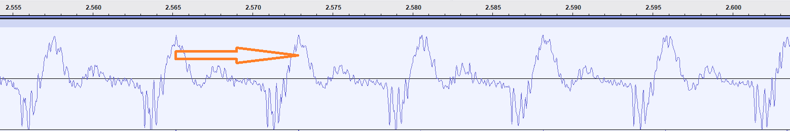
The period is approximately 0.00763 seconds; its reciprocal is about 131 Hz; looking up Wikipedia’s table of piano key frequencies, we can infer that Cat Stevens was singing a C3, the note one octave below middle C.

When I first started thinking about measuring pitch with a computer, I thought that the most natural approach was to take a Fourier transform of the signal (as discussed in a recent post), converting from the time domain to the frequency domain. Pitches are frequencies! But for a short 0.1-second clip, the FFT only shows frequency components for every 10 Hertz, which is a little larger than the gap between C3 and C♯ or B.

We have much finer resolution looking at the period: a typical audio track has 44,100 samples every second; a period of 336 samples means a frequency of 131.25 Hz, and a period of 337 samples is a frequency of 130.86 Hz, allowing a note to be cleanly identified, or evaluated as slightly sharp or flat.³

But the FFT will still turn out to be useful, performing a couple of supporting roles.

Pitch is not always frequency

I don’t know if the following experiment will work for you. It works for me when I listen to the video with headphones when played from VLC or Media Player. It doesn’t work when I play from Chrome, which modifies the audio somehow!! (I do get some brief hiccup, but it doesn’t illustrate what I’m about to describe.)

The video starts with a pure sine wave for middle C. I then gradually increase the amplitude of a second sine wave at 1.5 times the frequency, the note G in just intonation. For small amplitudes of the G, I hear only the harmony of the two notes. But when the amplitude of the G gets close to the amplitude of the C (above 0.8 or 0.9 or so), I suddenly hear a hum an octave below the C.

This is called a missing fundamental. Harmonics from an instrument are usually at frequencies that are integer multiples of the fundamental, which is the pitch that we perceive. If the two sine-wave frequencies are 300 Hz and 450 Hz, then there’s a missing fundamental at 150 Hz, an octave lower than the 300 Hz component. The period of the combined wave is the lowest common multiple of the two component periods.

One interesting aspect of this is that mathematically, the combined period becomes this lowest common multiple as soon as the amplitude of the second sine wave is non-zero, but I don’t hear the missing fundamental until the amplitude is quite large. “[P]itch is not a purely objective physical property; it is a subjective psychoacoustical attribute of sound,” says Wikipedia.

A program that uses the period of the sound waves alone to compute a pitch is therefore guaranteed to fail in at least some cases. But real-world instruments usually have fundamentals, so this section probably has no implications for my practical purposes.

Autocorrelation functions

Let x_n be a signal of length N, with n = 0, 1, …, N − 1. To find the period, we shift the signal by some number of samples, and compare it to the original. If we’re at a period, or an integer multiple of the period, then the original signal and its shifted (or lagged) cousin should look almost identical.

We can quantify this by calculating a sum of square differences for a lag of m samples, which I will call SSD before soon forgetting about it:

\(\mathrm{SSD}_m = \sum_{n=0}^{N-1} (x_n - x_{n-m})^2.\)

For ease of doing maths and programming, the indices wrap around, so that index N is identified with index 0 and index −1 with index N − 1. The signal will usually not vary smoothly across this boundary, so we are introducing some sort of noise or error into the calculation. But at the frequencies of interest in this post, it will not be a major concern: for my pitch graphs I use signals of length 4096 samples, and at 131 Hz for example, there will be plenty of full periods (1 period ≈ 337 samples) at the important lag inside the good part of the interval, and only a small percentage of the calculation will be spoiled by the wrap-around.

Expanding the SSD formula gives the decomposition

\(\begin{align} \mathrm{SSD}_m &= \sum_{n=0}^{N-1} (x_n - x_{n-m})^2 \\ &= \sum_{n=0}^{N-1} (x_n^2 + x_{n-m}^2 - 2x_n x_{n-m}) \\ &= 2 \sum_{n=0}^{N-1} x_n^2 - 2 \sum_{n=0}^{N-1} x_n x_{n-m}. \end{align}\)

The first of these two sums, over the squares of the signal values, does not vary with the lag. We can therefore ignore it as we test different lags, and focus only on the “cross” term between the signal and the lagged signal.

I will, perhaps loosely, call this sum of products an autocorrelation, though as written it is not normalised to between −1 and 1 as we would usually expect a correlation to be:

\(\rho_m = \sum_{n=0}^{N-1} x_n x_{n-m}.\)

We want this term to be high (we want the sum of square differences to be low, and the autocorrelation term was subtracted in the SSD expansion). As some intuition, when the waves align after a specific lag (so that we’re at the period, or an integer multiple of it), the positive elements of the signal array and the lagged signal will multiply together, and the negative parts of both will also multiply together to make positive numbers. But if the lagged signal is out of phase with the original signal, then we’d often be multiplying a positive number by a negative number, reducing (or making further negative) the autocorrelation at that lag.

Since we don’t know in advance what the period of the signal is, we will need to test many different lags. The calculation for one lag is an O(N) walk down the array, and if we calculate M lags, then a naive extrapolation makes this an O(NM) calculation, and O(N^2) if we systematically calculate all lags.

I knew that there was a faster alternative, and ChatGPT (5.2 Thinking) filled in the gaps in my memory. If x is the signal and X its FFT, then the autocorrelation is the inverse FFT of |X|^2. This fact is cited as the Wiener-Khinchin theorem, though the Wikipedia article talks about it in a more general and difficult context than a finite discrete signal.

For all I need of the theorem, its explanation follows from mechanical algebra and the orthogonality relation

\(\frac{1}{N} \sum_{n=0}^{N-1} \exp\left( \frac{i\tau n}{N}(k-k') \right) = \delta_{kk'},\)

which I stated in my previous Fourier post without formal proof but with much heartfelt conviction of its truthfulness.

We get the mod-square of a complex number by multiplying it by its complex conjugate, so

\(\begin{align} \mathrm{IFFT}(|X|^2)_m &= \frac{1}{N} \sum_{k=0}^{N-1} X_k \bar{X}_k \exp\left( \frac{i\tau k m}{N}\right) \\ &= \frac{1}{N} \sum_{k=0}^{N-1} \left( \sum_{n=0}^{N-1} x_n \exp\left( -\frac{i\tau k n}{N}\right) \right) \left( \sum_{p=0}^{N-1} x_p \exp\left( \frac{i\tau kp}{N}\right) \right) \exp\left( \frac{i\tau k m}{N}\right) \\ &= \frac{1}{N} \sum_{k,n,p=0}^{N-1} x_n x_p \exp\left( \frac{i\tau k}{N} ( m + p - n ) \right) \\ &= \sum_{n,p=0}^{N-1} x_n x_p \delta_{p,n-m} \\ &= \sum_{n=0}^{N-1} x_n x_{n-m} \\ &= \rho_m \end{align}\)

as required.

Since the FFT and its inverse are each O(N log(N)), and the only other operations in this sequence are linear in N, doing the calculation this way gives the autocorrelation for all possible lags in O(N log(N)) time.

Some graphs and nitty-gritty

As I built my pitch graph script, I quickly realised that there would be more steps required than “find the peak of the autocorrelation function”, most of them related to figuring out when not to process an audio snippet, because it didn’t represent a clear note.

One immediate complication is that the peak of the autocorrelation occurs when the lag is zero, because then the signal and the lagged signal are identical. So I only searched for the autocorrelation maximum at lags large enough to correspond to piano notes (very small non-zero lags correspond to extremely high frequencies). My graphs therefore all omit very short lags.

Here is a nice, easily interpretable autocorrelation function. The horizontal axis is the lag in samples; the units of the vertical axis don’t matter:

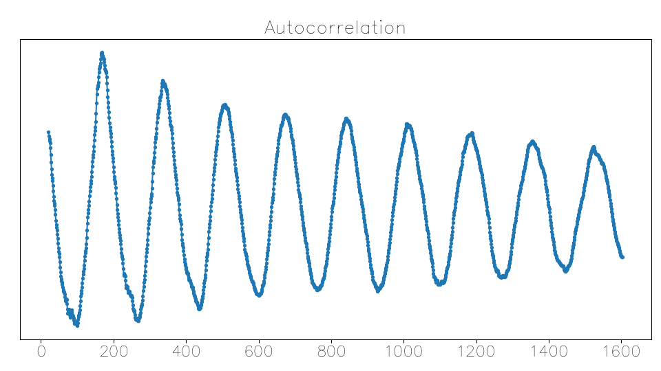
The strongest peak is the first local maximum; at larger lags the correlation decays; completely unambiguous. The period is about 168 samples, corresponding to about 262 Hz, C4.

But I wondered what would happen if the second peak was close in strength to the first peak. One of ChatGPT’s suggestions was to calculate the cepstrum (the spelling derived from reversing the letters of spec): instead of doing an inverse FFT on |X|^2, you do an inverse FFT on log(|X|^2). The reasoning, provided by ChatGPT and now imbued with human intentionality by me (I don’t quite really understand it though), is that the log makes the peaks in Fourier space more equal in magnitude, and the IFFT may then more prominently emphasise the regular spacing between the harmonics.

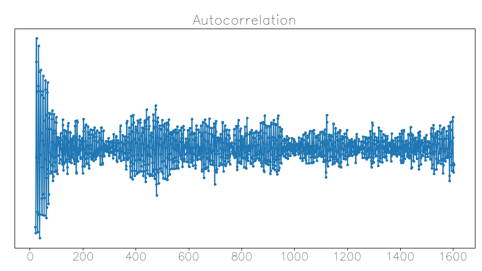
Here’s a case where interpreting the autocorrelation is very difficult, but the cepstrum gets it correct:

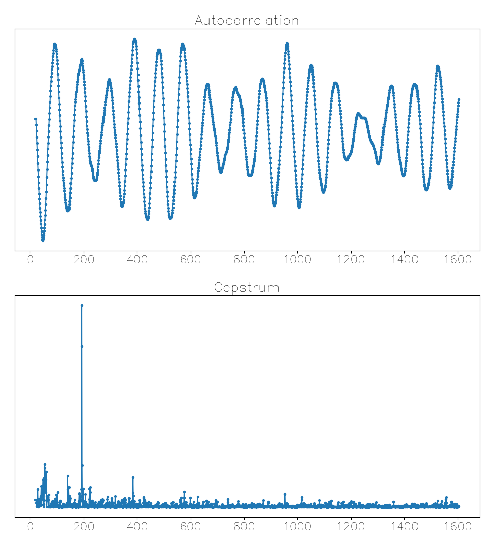
This is one of the snippets from the Springsteen example, where the pitch graph was jumping across octaves. The cepstrum peak is very clear and during this brief passage stays consistently around a lag of 200 samples, while the corresponding autocorrelation peak is not very prominent.

ChatGPT insisted that I shouldn’t think of the cepstrum peak as being at an autocorrelation lag, despite the numerical similarity – it gets called a quefrency,⁴ and the peak doesn’t necessarily correspond to a peak in the autocorrelation. Sadly, these admonishments were well-founded: in many cases the cepstrum maximum does not remotely resemble the perceived pitch, so despite its occasional success, my script always uses the autocorrelation alone.

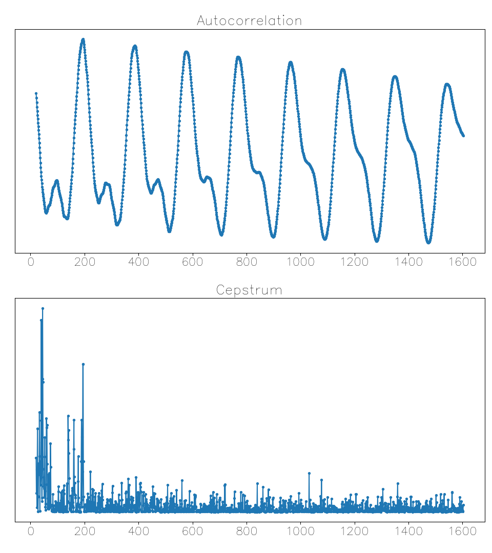
A few tenths of a second after the previous example, a useless early cepstrum maximum when the autocorrelation function gives the right answer:

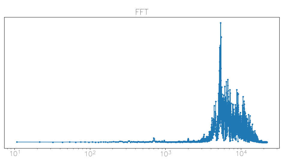
Something that I didn’t think of in advance, despite having observed it the last time I did some audio processing, is that an ‘s’ sound contains a lot of very high-frequency components. ‘Femininomenon’ starts with a sibilant, so I ran into this autocorrelation function quite early:

After realising what had happened, I decided to calculate a weighted log average of the FFT frequencies using |X|^2, skipping the processing if this average frequency was too high. Here is a sibilant FFT (horizontal axis is frequency), with lots of strong frequency components well over 1000 Hz:

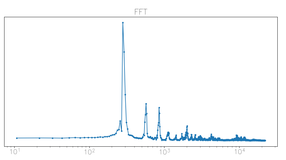
A vowel’s FFT:

I also skipped snippets whose volume seemed too low, calculating a decibel level by blindly trusting a ChatGPT-supplied log-RMS formula and manually adjusting the threshold as needed for each track.

Code

Once the libraries are imported, this code generates a static PNG for a 10-second audio clip very quickly, taking a second or so. If you output the detail plots (autocorrelation/cepstrum/FFT) or the movie frames, then it takes a few minutes on my computer.

# Plot pitch against time

import numpy as np
import matplotlib.pyplot as plt
from scipy.io import wavfile
import subprocess
from pathlib import Path

print("Finished imports")

wav_path = "vocals.wav"
title = "Pitch graph: "
title += "Singer"
title += " - Title"

output_png = "pitch_graph.png"

# On a new audio clip, set this
# to None and run without
# details or movie, and see if
# it needs adjusting
y_max = None

# Adjust as needed:
threshold_db = -30

# window size in samples:
N = 4096

# Plot increment on time axis:
dt = 0.02

# Range in which to search for
# the pitch:
freq_min = 27.5
freq_max = 2093.005

detail_path = Path("details")
movie_path = Path("frames")

plot_details = False
make_movie = False

# Framerate for the video:
fps = 60

eps = 1e-12
dpi = 96

movie_path.mkdir(exist_ok=True)
detail_path.mkdir(exist_ok=True)

def clear_dir(p):
  for f in p.iterdir():
    if f.is_file():
      f.unlink()

if plot_details:
  clear_dir(detail_path)

if make_movie:
  clear_dir(movie_path)

# sample rate, samples:
sr, x = wavfile.read(wav_path)

print("Read wav file")

# Plot increment in samples:
ds = int(sr * dt)

lag_hi = int(sr / freq_min) + 1
lag_lo = int(sr / freq_max)

lags = np.arange(
  lag_lo, lag_hi,
  dtype=np.int64
)

# We search for the autocorr
# peak within the lag slice:
lag_slice = slice(
  lag_lo, lag_hi
)

# Slice for FFT frequencies:
# in calculating the weighted
# log-freq, I ignore the
# constant, and don't go past
# the half-way point, when we
# wrap into (negative) lower
# frequencies.
freq_slice = slice(1, N // 2)

# The frequency axis for the
# FFT array:
fft_df = sr / N
fft_f = [
  fft_df * i
  for i in range(1, N // 2)
]

# Average stereo tracks to mono:
if x.ndim == 2:
  x = x.mean(axis=1)

# Convert to float (ChatGPT):
is_int = np.issubdtype(
  x.dtype, np.integer
)

if is_int:
  maxint = np.iinfo(x.dtype).max
  x = x.astype(np.float32)
  x /= maxint
else:
  x = x.astype(np.float32)

N_tot = len(x)

# Start of current window (in
# samples):
i0 = 0

# Lists that will hold the plot
# data:
plot_t = []
plot_freq = []
plot_cep = []

# Main loop through the track:
while i0 + N < N_tot:
  x_loc = x[i0:(i0 + N)]
  
  # Find volume (ChatGPT);
  # we'll skip if it's too quiet
  rms = np.sqrt(
    np.mean(x_loc**2)
  )

  rms_dbfs = 20 * np.log10(
    max(rms, eps)
  )

  plot_t.append(i0 / sr)
  plot_freq.append(np.nan)
  plot_cep.append(np.nan)

  x_fft = np.fft.fft(x_loc)
  mod_sq = np.abs(x_fft)**2
  
  # Check that most of the
  # sound is in the lower freqs

  wt = np.real(
    mod_sq[freq_slice]
  )
  
  mean_f = np.exp(
    np.sum(wt * np.log(fft_f))
    / np.sum(wt)
  )
  
  # Calculate autocorrelation:
  rho = np.real(
    np.fft.ifft(mod_sq)
  )

  # Calculate cepstrum:
  ifft_log = np.fft.ifft(
    np.log(mod_sq)
  )
  cep = np.abs(ifft_log)**2

  rho = rho[lag_slice]
  cep = cep[lag_slice]

  if plot_details:
    plt.close("all")
    fig, ax = plt.subplots(2,2)
    ax[0, 0].plot(
        lags, rho, ".-"
    )

    ax[0, 0].set_yticks(
      [], labels=[]
    )

    ax[0, 0].set_title(
      "Autocorrelation"
    )

    ax[1, 0].plot(
      lags, cep, ".-"
    )

    ax[1, 0].set_yticks(
      [], labels=[]
    )

    ax[1, 0].sharex(ax[0, 0])
    ax[1, 0].set_title(
      "Cepstrum"
    )

    ax[0, 1].plot(
      fft_f,
      np.abs(x_fft[freq_slice]),
      ".-"
    )

    ax[0, 1].set_xscale("log")
    ax[0, 1].set_title("FFT")
    ax[0, 1].set_yticks(
      [], labels=[]
    )

    ann = ax[1, 1]
    ann.axis("off")

    out_png = (
      detail_path /
      f"t_{plot_t[-1]:.2f}.png"
    )

    fig.set_size_inches(
      1920/dpi, 1080/dpi
    )
    fig.tight_layout()

  i0 += ds
  skip = False
  annots = [
    f"t = {plot_t[-1]:.2f}",
    f"Volume = {rms_dbfs:.1f}dB"
  ]
  
  if rms_dbfs < threshold_db:
    skip = True
    annots.append(
      "Volume too low."
    )

  if mean_f > freq_max:
    skip = True
    annots.append(
      "Too high frequency."
    )

  # Make sure we're past the
  # first minimum in the
  # autocorrelation, otherwise
  # maybe the first index is the
  # max.
  drho = rho[1:] - rho[:-1]
  increasing = np.where(
    drho > 0
  )[0]
  offset = increasing[0]
  
  rho = rho[offset:]
  cep = cep[offset:]

  cep_peak_i = np.argmax(cep)
  rho_peak_i = np.argmax(rho)

  if rho_peak_i < 3:
    skip = True
    annots.append(
      "Peak at too small lag."
    )
    continue

  local_sl = slice(
    rho_peak_i - 3,
    rho_peak_i + 4
  )

  local_rho = rho[local_sl]
  local_lags = lags[local_sl]

  a, b, c = np.polyfit(
    local_lags,
    local_rho,
    deg=2
  )

  peak = -b / (2*a) + offset
  if not skip:
    annots.append(
      f"peak lag = {peak:.2f}"
      + f", {sr/peak:.1f}Hz"
    )

  if plot_details:
    ann.text(
      0.5, 0.5,
      "\n".join(annots),
      ha="center",
      va="center",
      transform=ann.transAxes
    )
    fig.savefig(out_png,dpi=dpi)

  if skip:
    continue
  
  plot_freq[-1] = sr / peak
  plot_cep[-1] = (
    sr / lags[cep_peak_i]
  )

# Use music notes for the
# y-axis ticks
semitone = 2**(1/12)
note_freqs = [27.5]
tick_labels = ["A"]

notes = [
  "A", "", "B", "C", "", "D",
  "", "E", "F", "", "G", ""
]

octave = 0

for i in range(1, 88):
  note_freqs.append(
    note_freqs[-1] * semitone
  )

  note = notes[i % 12]
  if note == "C":
    octave += 1
    note += f"{octave}"
  tick_labels.append(note)


plt.close("all")

one_pixel = 72 / dpi
y_min = np.nanmin(plot_freq)

if y_max is None:
  y_max = np.nanmax(plot_freq)

fig, ax = plt.subplots()
ax.plot(
  plot_t, plot_freq,
  ".-", linewidth=one_pixel
)

ax.set_yscale("log")

ax.set_yticks(
  note_freqs,
  labels=tick_labels,
  minor=False
)

ax.set_yticks(
  [], labels = [], minor=True
)

ax.yaxis.grid(True)

ax.set_ylim(
  0.9 * y_min,
  1.1 * y_max
)

ax.set_xlabel("Time (s)")

fig.suptitle(title)

fig.set_size_inches(
  1280/dpi, 720/dpi
)

fig.tight_layout()
fig.savefig(output_png, dpi=dpi)

if make_movie:
  # Move a cursor across the
  # time axis
  max_t = plot_t[-1]
  n_frames = int(
    max_t * fps + 1
  )
    
  cursor = ax.axvline(
    0., lw = one_pixel,
    color = "black"
  )
  
  for i_f in range(n_frames):
    t = i_f / fps
    cursor.set_xdata([t, t])

    frame_path = (
      movie_path /
      f"frame{i_f:04d}.png"
    )

    fig.savefig(
      frame_path, dpi=dpi
    )
  
  frame_pattern = (
    f"{movie_path}" + 
    "/frame%04d.png"
  )

  ffmpeg_cmd = [
    "ffmpeg",
    "-y", # overwrite output
    "-framerate", f"{fps}",
    "-i", frame_pattern,
    "-i", wav_path,
    "-c:v", "libx264",
    "-pix_fmt", "yuv420p",
    "-c:a", "aac",
    "-b:a", "256k",
    "-shortest",
    wav_path.replace(
      "wav", "mp4"
    )
  ]
  
  subprocess.run(
    ffmpeg_cmd,
    check=True,
    capture_output=False,
    text=True
  )

1. I don’t have any particular recommendations on that page. He has a formula and, at least in the videos I’ve watched, he sticks to it.

2. While I’m not shocked that sometimes my code goes an octave high, for the reasons stated in the previous paragraph, I’m nevertheless still mildly surprised that this happens. A priori, I’d expect to get a lot more errors of the second type, calculating double-periods instead of single-periods and being an octave low.

3. The balance of this consideration may change at much higher frequencies, such as those in Mariah Carey’s whistle register. At the top of her range, there’d only be about 15 samples per period in a 44.1 kHz recording, and the accuracy of the period determination would depend on interpolating a curve between integer numbers of samples. Meanwhile an FFT’s 10-Hz intervals are much smaller than a semitone interval for notes that high. I haven’t run any experiments on this though.

4. Bogert, Healy, and Tukey evidently having too much of a sense of humour.